Difference between revisions of "Subtangent and subnormal"
(Importing text file) |
|||
| (One intermediate revision by one other user not shown) | |||
| Line 1: | Line 1: | ||
| − | + | <!-- | |
| + | s0910401.png | ||
| + | $#A+1 = 14 n = 0 | ||
| + | $#C+1 = 14 : ~/encyclopedia/old_files/data/S091/S.0901040 Subtangent and subnormal | ||
| + | Automatically converted into TeX, above some diagnostics. | ||
| + | Please remove this comment and the {{TEX|auto}} line below, | ||
| + | if TeX found to be correct. | ||
| + | --> | ||
| + | |||
| + | {{TEX|auto}} | ||
| + | {{TEX|done}} | ||
| + | |||
| + | The directed segments $ QT $ | ||
| + | and $ QN $ | ||
| + | which are the projections on the $ x $- | ||
| + | axis of the segments of the [[Tangent line|tangent line]] $ MT $ | ||
| + | and the [[Normal|normal]] $ MN $ | ||
| + | to a certain curve at a point $ M $( | ||
| + | see Fig.). | ||
<img style="border:1px solid;" src="https://www.encyclopediaofmath.org/legacyimages/common_img/s091040a.gif" /> | <img style="border:1px solid;" src="https://www.encyclopediaofmath.org/legacyimages/common_img/s091040a.gif" /> | ||
| Line 5: | Line 23: | ||
Figure: s091040a | Figure: s091040a | ||
| − | If the curve is the graph of a function | + | If the curve is the graph of a function $ y = f( x) $, |
| + | the values of the subtangent and subnormal are equal to | ||
| − | + | $$ | |
| + | QT = - | ||
| + | \frac{f( x) }{f ^ { \prime } ( x) } | ||
| + | ,\ \ | ||
| + | ON = f( x) f ^ { \prime } ( x), | ||
| + | $$ | ||
| − | respectively, where | + | respectively, where $ x $ |
| + | is the abscissa of the point $ M $. | ||
| + | If the curve is given parametrically by | ||
| − | + | $$ | |
| + | x = \phi ( t),\ y = \psi ( t), | ||
| + | $$ | ||
then | then | ||
| − | + | $$ | |
| + | QT = - | ||
| + | \frac{\psi ( t) \phi ^ \prime ( t) }{\psi ^ \prime ( t) } | ||
| + | ,\ \ | ||
| + | QN = | ||
| + | \frac{\psi ( t) \psi ^ \prime ( t) }{\psi ^ \prime ( t) } | ||
| + | , | ||
| + | $$ | ||
| − | where | + | where $ t $ |
| + | is the value of the parameter defining the point $ M $ | ||
| + | on the curve. | ||
| + | ====References==== | ||
| + | <table> | ||
| + | <TR><TD valign="top">[a1]</TD> <TD valign="top"> M. Berger, "Geometry" , '''II''' , Springer (1989)</TD></TR><TR><TD valign="top">[a2]</TD> <TD valign="top"> F. Gomes Teixeira, "Traité des courbes" , '''1–3''' , Chelsea, reprint (1971)</TD></TR><TR><TD valign="top">[a3]</TD> <TD valign="top"> H. Lamb, "Infinitesimal calculus" , Cambridge (1924) pp. 118</TD></TR> | ||
| + | </table> | ||
| − | + | {{OldImage}} | |
| − | |||
| − | |||
| − | |||
| − | |||
Latest revision as of 18:38, 13 May 2023
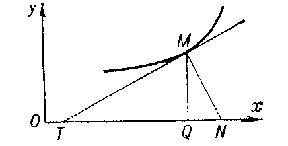
The directed segments $ QT $
and $ QN $
which are the projections on the $ x $-
axis of the segments of the tangent line $ MT $
and the normal $ MN $
to a certain curve at a point $ M $(
see Fig.).

Figure: s091040a
If the curve is the graph of a function $ y = f( x) $, the values of the subtangent and subnormal are equal to
$$ QT = - \frac{f( x) }{f ^ { \prime } ( x) } ,\ \ ON = f( x) f ^ { \prime } ( x), $$
respectively, where $ x $ is the abscissa of the point $ M $. If the curve is given parametrically by
$$ x = \phi ( t),\ y = \psi ( t), $$
then
$$ QT = - \frac{\psi ( t) \phi ^ \prime ( t) }{\psi ^ \prime ( t) } ,\ \ QN = \frac{\psi ( t) \psi ^ \prime ( t) }{\psi ^ \prime ( t) } , $$
where $ t $ is the value of the parameter defining the point $ M $ on the curve.
References
| [a1] | M. Berger, "Geometry" , II , Springer (1989) |
| [a2] | F. Gomes Teixeira, "Traité des courbes" , 1–3 , Chelsea, reprint (1971) |
| [a3] | H. Lamb, "Infinitesimal calculus" , Cambridge (1924) pp. 118 |
Subtangent and subnormal. Encyclopedia of Mathematics. URL: http://encyclopediaofmath.org/index.php?title=Subtangent_and_subnormal&oldid=14018