Difference between revisions of "Zak transform"
(Importing text file) |
m (AUTOMATIC EDIT (latexlist): Replaced 74 formulas out of 80 by TEX code with an average confidence of 2.0 and a minimal confidence of 2.0.) |
||
| Line 1: | Line 1: | ||
| − | + | <!--This article has been texified automatically. Since there was no Nroff source code for this article, | |
| + | the semi-automatic procedure described at https://encyclopediaofmath.org/wiki/User:Maximilian_Janisch/latexlist | ||
| + | was used. | ||
| + | If the TeX and formula formatting is correct, please remove this message and the {{TEX|semi-auto}} category. | ||
| + | |||
| + | Out of 80 formulas, 74 were replaced by TEX code.--> | ||
| + | |||
| + | {{TEX|semi-auto}}{{TEX|partial}} | ||
| + | ''Gel'fand mapping, $k$-$q$ representation, Weil–Brezin mapping'' | ||
The Zak transform was discovered by several people in different fields and was called by different names, depending on the field in which it was discovered. It was called the "Gel'fand mapping" in the Russian literature because I.M. Gel'fand [[#References|[a3]]] introduced it in his work on eigenfunction expansions associated with Schrödinger operators with periodic potentials. In 1967, almost 17 years after the publication of Gel'fand's work, the transform was rediscovered independently by a solid-state physicist, J. Zak, who called it the "k-q representation" . Zak introduced this representation to construct a quantum-mechanical representation for the motion of a Bloch electron in the presence of a magnetic or electric field [[#References|[a8]]], [[#References|[a9]]]. It has also been said [[#References|[a7]]] that some properties of another version of the Zak transform, called the "Weil–Brezin mapping" in [[#References|[a1]]], [[#References|[a7]]], were even known to the mathematician C.F. Gauss. Nevertheless, there seems to be a general consent among experts in the field to call it the Zak transform, since Zak was indeed the first to systematically study that transform in a more general setting and recognize its usefulness. | The Zak transform was discovered by several people in different fields and was called by different names, depending on the field in which it was discovered. It was called the "Gel'fand mapping" in the Russian literature because I.M. Gel'fand [[#References|[a3]]] introduced it in his work on eigenfunction expansions associated with Schrödinger operators with periodic potentials. In 1967, almost 17 years after the publication of Gel'fand's work, the transform was rediscovered independently by a solid-state physicist, J. Zak, who called it the "k-q representation" . Zak introduced this representation to construct a quantum-mechanical representation for the motion of a Bloch electron in the presence of a magnetic or electric field [[#References|[a8]]], [[#References|[a9]]]. It has also been said [[#References|[a7]]] that some properties of another version of the Zak transform, called the "Weil–Brezin mapping" in [[#References|[a1]]], [[#References|[a7]]], were even known to the mathematician C.F. Gauss. Nevertheless, there seems to be a general consent among experts in the field to call it the Zak transform, since Zak was indeed the first to systematically study that transform in a more general setting and recognize its usefulness. | ||
| − | The Zak transform | + | The Zak transform $Z _ { a } ( f )$ of a function $f$ is defined by |
| − | <table class="eq" style="width:100%;"> <tr><td | + | <table class="eq" style="width:100%;"> <tr><td style="width:94%;text-align:center;" valign="top"><img align="absmiddle" border="0" src="https://www.encyclopediaofmath.org/legacyimages/z/z130/z130030/z1300307.png"/></td> <td style="width:5%;text-align:right;" valign="top">(a1)</td></tr></table> |
| − | + | \begin{equation*} = \sqrt { a } \sum _ { k = - \infty } ^ { \infty } f ( a t + a k ) e ^ { - 2 \pi i k w }, \end{equation*} | |
| − | where | + | where $a > 0$ and $t$ and $w$ are real. When $a = 1$, one denotes $Z _ { a } f$ by $Z f$. |
| − | If | + | If $f$ represents a signal, then its Zak transform can be considered as a mixed time-frequency representation of $f$, and it can also be considered as a generalization of the discrete Fourier transform of $f$ in which an infinite sequence of samples in the form $f ( a t + a k )$, $k = 0 , \pm 1 , \pm 2 , \ldots$, is used (cf. also [[Fourier transform|Fourier transform]]). |
==Examples.== | ==Examples.== | ||
| − | If | + | If $a = 1$ and $f ( t ) = 0$ outside $[ - b , b ]$, $0 < b \leq 1 / 2$, then $( Z f ) ( t , w ) = f ( t )$, $| t | \leq 1 / 2$. |
The Zak transform of the Gaussian function | The Zak transform of the Gaussian function | ||
| − | + | \begin{equation*} f ( t ) = ( 2 \gamma ) ^ { 1 / 4 } \operatorname { exp } ( - \pi \gamma t ^ { 2 } ) , \gamma > 0, \end{equation*} | |
is easily shown to be | is easily shown to be | ||
| − | + | \begin{equation*} ( Z f ) ( t , w ) = ( 2 \gamma ) ^ { 1 / 4 } e ^ { - \pi \gamma t ^ { 2 } } \theta _ { 3 } ( w - i \gamma t , e ^ { - \pi \gamma } ), \end{equation*} | |
| − | where | + | where $\theta _ { 3 }$ is the third theta-function, defined by |
| − | + | \begin{equation*} \theta _ { 3 } ( z , q ) = \sum _ { k = - \infty } ^ { \infty } q ^ { k ^ { 2 } } e ^ { - 2 \pi i k z }. \end{equation*} | |
==Existence.== | ==Existence.== | ||
| − | If | + | If $f$ is integrable or square integrable (cf. [[Integrable function|Integrable function]]), its Zak transform exists almost everywhere. In particular, if $f$ is a [[Continuous function|continuous function]] such that $| f ( t ) | \leq C ( 1 + | t | ) ^ { - (1 + \epsilon ) }$, for some $\epsilon > 0$, for all $t$, then its Zak transform exists and defines a continuous function. |
==Elementary properties.== | ==Elementary properties.== | ||
| − | 1) (linearity): for any complex numbers | + | 1) (linearity): for any complex numbers $a$ and $b$, |
| − | + | \begin{equation*} Z [ a f ( t ) + b g ( t ) ] ( t , w ) = a Z [ f ( t ) ] ( t , w ) + b Z [ g ( t ) ] ( t , w ). \end{equation*} | |
| − | 2) (translation): for any integer | + | 2) (translation): for any integer $m$, |
| − | + | \begin{equation*} Z [ f ( t + m ) ] ( t , w ) = e ^ { 2 \pi i m w } Z [ f ] ( t , w ); \end{equation*} | |
in particular, | in particular, | ||
| − | + | \begin{equation*} ( Z f ) ( t + 1 , w ) = e ^ { 2 \pi i w } ( Z f ) ( t , w ). \end{equation*} | |
3) (modulation): | 3) (modulation): | ||
| − | + | \begin{equation*} Z [ e ^ { 2 \pi i m t } f ] ( t , w ) = e ^ { 2 \pi i m t } ( Z f ) ( t , w ). \end{equation*} | |
| − | 4) (periodicity): The Zak transform is periodic in | + | 4) (periodicity): The Zak transform is periodic in $w$ with period one, that is, |
| − | + | \begin{equation*} ( Z f ) ( t , w + 1 ) = ( Z f ) ( t , w ). \end{equation*} | |
5) (translation and modulation): By combining 2) and 3) one obtains | 5) (translation and modulation): By combining 2) and 3) one obtains | ||
| − | + | \begin{equation*} Z \left[ e ^ { 2 \pi i m t } f ( t + n ) \right] ( t , w ) = e ^ { 2 \pi i m t } e ^ { 2 \pi i n w } ( Z f ) ( t , w ). \end{equation*} | |
6) (conjugation): | 6) (conjugation): | ||
| − | + | \begin{equation*} ( Z \overline { f } ) ( t , w ) = \overline { ( Z f ) } ( t , - w ). \end{equation*} | |
| − | 7) (symmetry): If | + | 7) (symmetry): If $f$ is even (cf. also [[Even function|Even function]]), then |
| − | + | \begin{equation*} ( Z f ) ( t , w ) = ( Z f ) ( - t , - w ), \end{equation*} | |
| − | and if | + | and if $f$ is odd, then |
| − | + | \begin{equation*} ( Z f ) ( t , w ) = - ( Z f ) ( - t , - w ). \end{equation*} | |
| − | From 6) and 7) it follows that if | + | From 6) and 7) it follows that if $f$ is real-valued and even, then |
| − | + | \begin{equation*} ( Z f ) ( t , w ) = \overline { ( Z f ) } ( t , - w ) = ( Z f ) ( - t , - w ). \end{equation*} | |
| − | Because of 2) and 4), the Zak transform is completely determined by its values on the unit square | + | Because of 2) and 4), the Zak transform is completely determined by its values on the unit square $Q = [ 0,1 ] \times [ 0,1 ]$. |
8) (convolution): Let | 8) (convolution): Let | ||
| − | + | \begin{equation*} h ( t ) = \int _ { - \infty } ^ { \infty } R ( t - s ) f ( s ) d s; \end{equation*} | |
then | then | ||
| − | + | \begin{equation*} ( Z h ) ( t , w ) = \int _ { 0 } ^ { 1 } ( Z R ) ( t - s , w ) ( Z f ) ( s , w ) d s. \end{equation*} | |
==Analytic properties.== | ==Analytic properties.== | ||
| − | If | + | If $f$ is a continuous function such that $f ( t ) = O \left( ( 1 + | t | ) ^ { - 1 - \epsilon } \right)$ as $| t | \rightarrow \infty$ for some $\epsilon > 0$, then $Z f$ is continuous on $Q$. A rather peculiar property of the Zak transform is that if $Z f$ is continuous, it must have a zero in $Q$. The Zak transform is a [[Unitary transformation|unitary transformation]] from $L ^ { 2 } ( \mathcal{R} )$ onto $L ^ { 2 } ( Q )$; see [[#References|[a10]]], p. 481. |
==Inversion formulas.== | ==Inversion formulas.== | ||
The following inversion formulas for the Zak transform follow easily from the definition, provided that the series defining the Zak transform converges uniformly (cf. also [[Uniform convergence|Uniform convergence]]): | The following inversion formulas for the Zak transform follow easily from the definition, provided that the series defining the Zak transform converges uniformly (cf. also [[Uniform convergence|Uniform convergence]]): | ||
| − | + | \begin{equation*} f ( t ) = \int _ { 0 } ^ { 1 } ( Z f ) ( t , w ) d w , - \infty < t < \infty, \end{equation*} | |
| − | + | \begin{equation*} \hat { f } ( - 2 \pi w ) = \frac { 1 } { \sqrt { 2 \pi } } \int _ { 0 } ^ { 1 } e ^ { - 2 \pi i w t } ( Z f ) ( t , w ) d t, \end{equation*} | |
and | and | ||
| − | + | \begin{equation*} f ( 2 \pi t ) = \frac { 1 } { \sqrt { 2 \pi } } \int _ { 0 } ^ { 1 } e ^ { - 2 \pi i x t } ( Z \widehat { f } ) ( x , t ) d x, \end{equation*} | |
| − | where | + | where $\hat { f }$ is the [[Fourier transform|Fourier transform]] of $f$, given by |
| − | + | \begin{equation*} \hat { f } ( w ) = \frac { 1 } { \sqrt { 2 \pi } } \int _ { - \infty } ^ { \infty } f ( x ) e ^ { i w x } d x. \end{equation*} | |
==Applications.== | ==Applications.== | ||
The Zak transform has been used successfully in various applications in physics, such as in the study of the coherent states representation in [[Quantum field theory|quantum field theory]] [[#References|[a6]]], and in electrical engineering, such as in time-frequency representation of signals and in digital data transmission; see [[#References|[a4]]], [[#References|[a5]]]. | The Zak transform has been used successfully in various applications in physics, such as in the study of the coherent states representation in [[Quantum field theory|quantum field theory]] [[#References|[a6]]], and in electrical engineering, such as in time-frequency representation of signals and in digital data transmission; see [[#References|[a4]]], [[#References|[a5]]]. | ||
| − | The applications of the Zak transform are not limited to only physics and engineering. More recent applications of it in mathematics have proved to be very useful; in particular, to simplify proofs of some important results. A case in point is the Gabor representation problem. The Gabor representation problem can be stated as follows: Given | + | The applications of the Zak transform are not limited to only physics and engineering. More recent applications of it in mathematics have proved to be very useful; in particular, to simplify proofs of some important results. A case in point is the Gabor representation problem. The Gabor representation problem can be stated as follows: Given $g \in L ^ { 2 } ( \mathcal{R} )$ and two real numbers, $a$, $b,$ different from zero, is it possible to represent any function $f \in L ^ { 2 } ( \mathcal{R} )$ by a series of the form |
| − | <table class="eq" style="width:100%;"> <tr><td | + | <table class="eq" style="width:100%;"> <tr><td style="width:94%;text-align:center;" valign="top"><img align="absmiddle" border="0" src="https://www.encyclopediaofmath.org/legacyimages/z/z130/z130030/z13003075.png"/></td> </tr></table> |
| − | where | + | where $g_{mb , na}$ are the Gabor functions, defined by |
| − | <table class="eq" style="width:100%;"> <tr><td | + | <table class="eq" style="width:100%;"> <tr><td style="width:94%;text-align:center;" valign="top"><img align="absmiddle" border="0" src="https://www.encyclopediaofmath.org/legacyimages/z/z130/z130030/z13003077.png"/></td> </tr></table> |
| − | and | + | and $c_{m,n}$ are constants? And under what conditions is the representation unique? |
| − | The Zak transform has been used successfully to study the orthogonality and the completeness of Gabor frames in the crucial case where | + | The Zak transform has been used successfully to study the orthogonality and the completeness of Gabor frames in the crucial case where $a b = 1$; see [[#References|[a2]]], [[#References|[a10]]]. |
====References==== | ====References==== | ||
| − | <table>< | + | <table><tr><td valign="top">[a1]</td> <td valign="top"> L. Auslander, R. Tolimieri, "Radar ambiguity functions and group theory" ''SIAM J. Math. Anal.'' , '''16''' (1985) pp. 577–601</td></tr><tr><td valign="top">[a2]</td> <td valign="top"> I. Daubechies, "Ten lectures on wavelets" , SIAM (1992)</td></tr><tr><td valign="top">[a3]</td> <td valign="top"> I. Gel'fand, "Eigenfunction expansions for an equation with periodic coefficients" ''Dokl. Akad. Nauk. SSR'' , '''76''' (1950) pp. 1117–1120 (In Russian)</td></tr><tr><td valign="top">[a4]</td> <td valign="top"> A.J. Janssen, "The Zak transform: A signal transform for sampled time-continuous signals" ''Philips J. Research'' , '''43''' (1988) pp. 23–69</td></tr><tr><td valign="top">[a5]</td> <td valign="top"> A.J. Janssen, "Bargmann transform, Zak transform, and coherent states" ''J. Math. Phys.'' , '''23''' (1982) pp. 720–731</td></tr><tr><td valign="top">[a6]</td> <td valign="top"> J. Klauder, B.S. Skagerstam, "Coherent states" , World Sci. (1985)</td></tr><tr><td valign="top">[a7]</td> <td valign="top"> W. Schempp, "Radar ambiguity functions, the Heisenberg group and holomorphic theta series" ''Proc. Amer. Math. Soc.'' , '''92''' (1984) pp. 103–110</td></tr><tr><td valign="top">[a8]</td> <td valign="top"> J. Zak, "Finite translation in solid state physics" ''Phys. Rev. Lett.'' , '''19''' (1967) pp. 1385–1397</td></tr><tr><td valign="top">[a9]</td> <td valign="top"> J. Zak, "Dynamics of electrons in solids in external fields" ''Phys. Rev.'' , '''168''' (1968) pp. 686–695</td></tr><tr><td valign="top">[a10]</td> <td valign="top"> A.I. Zayed, "Function and generalized function transformations" , CRC (1996)</td></tr></table> |
Revision as of 16:57, 1 July 2020
Gel'fand mapping, $k$-$q$ representation, Weil–Brezin mapping
The Zak transform was discovered by several people in different fields and was called by different names, depending on the field in which it was discovered. It was called the "Gel'fand mapping" in the Russian literature because I.M. Gel'fand [a3] introduced it in his work on eigenfunction expansions associated with Schrödinger operators with periodic potentials. In 1967, almost 17 years after the publication of Gel'fand's work, the transform was rediscovered independently by a solid-state physicist, J. Zak, who called it the "k-q representation" . Zak introduced this representation to construct a quantum-mechanical representation for the motion of a Bloch electron in the presence of a magnetic or electric field [a8], [a9]. It has also been said [a7] that some properties of another version of the Zak transform, called the "Weil–Brezin mapping" in [a1], [a7], were even known to the mathematician C.F. Gauss. Nevertheless, there seems to be a general consent among experts in the field to call it the Zak transform, since Zak was indeed the first to systematically study that transform in a more general setting and recognize its usefulness.
The Zak transform $Z _ { a } ( f )$ of a function $f$ is defined by
 | (a1) |
\begin{equation*} = \sqrt { a } \sum _ { k = - \infty } ^ { \infty } f ( a t + a k ) e ^ { - 2 \pi i k w }, \end{equation*}
where $a > 0$ and $t$ and $w$ are real. When $a = 1$, one denotes $Z _ { a } f$ by $Z f$.
If $f$ represents a signal, then its Zak transform can be considered as a mixed time-frequency representation of $f$, and it can also be considered as a generalization of the discrete Fourier transform of $f$ in which an infinite sequence of samples in the form $f ( a t + a k )$, $k = 0 , \pm 1 , \pm 2 , \ldots$, is used (cf. also Fourier transform).
Examples.
If $a = 1$ and $f ( t ) = 0$ outside $[ - b , b ]$, $0 < b \leq 1 / 2$, then $( Z f ) ( t , w ) = f ( t )$, $| t | \leq 1 / 2$.
The Zak transform of the Gaussian function
\begin{equation*} f ( t ) = ( 2 \gamma ) ^ { 1 / 4 } \operatorname { exp } ( - \pi \gamma t ^ { 2 } ) , \gamma > 0, \end{equation*}
is easily shown to be
\begin{equation*} ( Z f ) ( t , w ) = ( 2 \gamma ) ^ { 1 / 4 } e ^ { - \pi \gamma t ^ { 2 } } \theta _ { 3 } ( w - i \gamma t , e ^ { - \pi \gamma } ), \end{equation*}
where $\theta _ { 3 }$ is the third theta-function, defined by
\begin{equation*} \theta _ { 3 } ( z , q ) = \sum _ { k = - \infty } ^ { \infty } q ^ { k ^ { 2 } } e ^ { - 2 \pi i k z }. \end{equation*}
Existence.
If $f$ is integrable or square integrable (cf. Integrable function), its Zak transform exists almost everywhere. In particular, if $f$ is a continuous function such that $| f ( t ) | \leq C ( 1 + | t | ) ^ { - (1 + \epsilon ) }$, for some $\epsilon > 0$, for all $t$, then its Zak transform exists and defines a continuous function.
Elementary properties.
1) (linearity): for any complex numbers $a$ and $b$,
\begin{equation*} Z [ a f ( t ) + b g ( t ) ] ( t , w ) = a Z [ f ( t ) ] ( t , w ) + b Z [ g ( t ) ] ( t , w ). \end{equation*}
2) (translation): for any integer $m$,
\begin{equation*} Z [ f ( t + m ) ] ( t , w ) = e ^ { 2 \pi i m w } Z [ f ] ( t , w ); \end{equation*}
in particular,
\begin{equation*} ( Z f ) ( t + 1 , w ) = e ^ { 2 \pi i w } ( Z f ) ( t , w ). \end{equation*}
3) (modulation):
\begin{equation*} Z [ e ^ { 2 \pi i m t } f ] ( t , w ) = e ^ { 2 \pi i m t } ( Z f ) ( t , w ). \end{equation*}
4) (periodicity): The Zak transform is periodic in $w$ with period one, that is,
\begin{equation*} ( Z f ) ( t , w + 1 ) = ( Z f ) ( t , w ). \end{equation*}
5) (translation and modulation): By combining 2) and 3) one obtains
\begin{equation*} Z \left[ e ^ { 2 \pi i m t } f ( t + n ) \right] ( t , w ) = e ^ { 2 \pi i m t } e ^ { 2 \pi i n w } ( Z f ) ( t , w ). \end{equation*}
6) (conjugation):
\begin{equation*} ( Z \overline { f } ) ( t , w ) = \overline { ( Z f ) } ( t , - w ). \end{equation*}
7) (symmetry): If $f$ is even (cf. also Even function), then
\begin{equation*} ( Z f ) ( t , w ) = ( Z f ) ( - t , - w ), \end{equation*}
and if $f$ is odd, then
\begin{equation*} ( Z f ) ( t , w ) = - ( Z f ) ( - t , - w ). \end{equation*}
From 6) and 7) it follows that if $f$ is real-valued and even, then
\begin{equation*} ( Z f ) ( t , w ) = \overline { ( Z f ) } ( t , - w ) = ( Z f ) ( - t , - w ). \end{equation*}
Because of 2) and 4), the Zak transform is completely determined by its values on the unit square $Q = [ 0,1 ] \times [ 0,1 ]$.
8) (convolution): Let
\begin{equation*} h ( t ) = \int _ { - \infty } ^ { \infty } R ( t - s ) f ( s ) d s; \end{equation*}
then
\begin{equation*} ( Z h ) ( t , w ) = \int _ { 0 } ^ { 1 } ( Z R ) ( t - s , w ) ( Z f ) ( s , w ) d s. \end{equation*}
Analytic properties.
If $f$ is a continuous function such that $f ( t ) = O \left( ( 1 + | t | ) ^ { - 1 - \epsilon } \right)$ as $| t | \rightarrow \infty$ for some $\epsilon > 0$, then $Z f$ is continuous on $Q$. A rather peculiar property of the Zak transform is that if $Z f$ is continuous, it must have a zero in $Q$. The Zak transform is a unitary transformation from $L ^ { 2 } ( \mathcal{R} )$ onto $L ^ { 2 } ( Q )$; see [a10], p. 481.
Inversion formulas.
The following inversion formulas for the Zak transform follow easily from the definition, provided that the series defining the Zak transform converges uniformly (cf. also Uniform convergence):
\begin{equation*} f ( t ) = \int _ { 0 } ^ { 1 } ( Z f ) ( t , w ) d w , - \infty < t < \infty, \end{equation*}
\begin{equation*} \hat { f } ( - 2 \pi w ) = \frac { 1 } { \sqrt { 2 \pi } } \int _ { 0 } ^ { 1 } e ^ { - 2 \pi i w t } ( Z f ) ( t , w ) d t, \end{equation*}
and
\begin{equation*} f ( 2 \pi t ) = \frac { 1 } { \sqrt { 2 \pi } } \int _ { 0 } ^ { 1 } e ^ { - 2 \pi i x t } ( Z \widehat { f } ) ( x , t ) d x, \end{equation*}
where $\hat { f }$ is the Fourier transform of $f$, given by
\begin{equation*} \hat { f } ( w ) = \frac { 1 } { \sqrt { 2 \pi } } \int _ { - \infty } ^ { \infty } f ( x ) e ^ { i w x } d x. \end{equation*}
Applications.
The Zak transform has been used successfully in various applications in physics, such as in the study of the coherent states representation in quantum field theory [a6], and in electrical engineering, such as in time-frequency representation of signals and in digital data transmission; see [a4], [a5].
The applications of the Zak transform are not limited to only physics and engineering. More recent applications of it in mathematics have proved to be very useful; in particular, to simplify proofs of some important results. A case in point is the Gabor representation problem. The Gabor representation problem can be stated as follows: Given $g \in L ^ { 2 } ( \mathcal{R} )$ and two real numbers, $a$, $b,$ different from zero, is it possible to represent any function $f \in L ^ { 2 } ( \mathcal{R} )$ by a series of the form
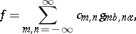 |
where $g_{mb , na}$ are the Gabor functions, defined by
 |
and $c_{m,n}$ are constants? And under what conditions is the representation unique?
The Zak transform has been used successfully to study the orthogonality and the completeness of Gabor frames in the crucial case where $a b = 1$; see [a2], [a10].
References
| [a1] | L. Auslander, R. Tolimieri, "Radar ambiguity functions and group theory" SIAM J. Math. Anal. , 16 (1985) pp. 577–601 |
| [a2] | I. Daubechies, "Ten lectures on wavelets" , SIAM (1992) |
| [a3] | I. Gel'fand, "Eigenfunction expansions for an equation with periodic coefficients" Dokl. Akad. Nauk. SSR , 76 (1950) pp. 1117–1120 (In Russian) |
| [a4] | A.J. Janssen, "The Zak transform: A signal transform for sampled time-continuous signals" Philips J. Research , 43 (1988) pp. 23–69 |
| [a5] | A.J. Janssen, "Bargmann transform, Zak transform, and coherent states" J. Math. Phys. , 23 (1982) pp. 720–731 |
| [a6] | J. Klauder, B.S. Skagerstam, "Coherent states" , World Sci. (1985) |
| [a7] | W. Schempp, "Radar ambiguity functions, the Heisenberg group and holomorphic theta series" Proc. Amer. Math. Soc. , 92 (1984) pp. 103–110 |
| [a8] | J. Zak, "Finite translation in solid state physics" Phys. Rev. Lett. , 19 (1967) pp. 1385–1397 |
| [a9] | J. Zak, "Dynamics of electrons in solids in external fields" Phys. Rev. , 168 (1968) pp. 686–695 |
| [a10] | A.I. Zayed, "Function and generalized function transformations" , CRC (1996) |
Zak transform. Encyclopedia of Mathematics. URL: http://encyclopediaofmath.org/index.php?title=Zak_transform&oldid=16833