A branch of mathematics in which functions are studied under a discrete change of the argument, as opposed to differential and integral calculus, where the argument changes continuously. Let  be a function defined at the points
  (where
  is a constant and
  is an integer). Then
are the (finite) first-order differences,
are the second-order differences
are the  -th order differences. The differences are conveniently arranged in a table:
An  -th order difference can be expressed in terms of the quantities
  by the formula
As well as the forward differences  , one uses the backward differences:
In a number of problems (in particular in the construction of interpolation formulas) central differences are used:
which are defined as follows:
The central differences  and the ordinary differences
  are related by the formula
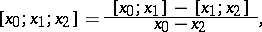
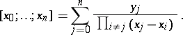
In the case when the intervals  are not of constant size, one also considers divided differences:
The following formula holds:
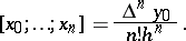
Sometimes, instead of  the notation
  is used. If
  ,
,  then
then
If  has an
  -th derivative
  throughout the interval
  , then
The calculus of finite differences is closely related to the general theory of approximation of functions, and is used in approximate differentiation and integration and in the approximate solution of differential equations, as well as in other questions. Suppose that the problem is posed (an interpolation problem) on recovering a function  from the known values of
  at points
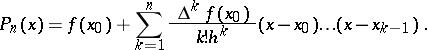
  . One constructs the interpolation polynomial
  of degree
  having the same values as
  at the indicated points. It can be expressed in various forms: in the form of Lagrange, Newton, etc. In Newton's form it is:
and in the case when the values of the independent variable are equally spaced:
The function  is set approximately equal to
  . If
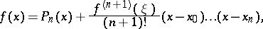
. If  has a derivative of order
  , then the error in replacing
  by
by  can be estimated by the formula
where  lies in the interval in which the points
  ly. If
  is a polynomial of degree
  , then
  .
.
As the number of nodes increases without bound, the interpolation polynomial  becomes in the limit a polynomial
  of "infinite" degree, and the following question naturally arises: When does
  ? In other words, when does the following equation hold:
 | (1) |
(for simplicity, the case of equally-spaced intervals is considered)? Let  ,
,  , so that
  (
( ). If the series (1) converges at a point
  that is not a node (the series (1) always converges at the nodes
  ), then it converges in the half-plane
  and is an analytic function in this half-plane which satisfies the following condition in any half-plane
  (where
  ):
):
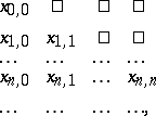
Conversely, if  is analytic in some half-plane and has similar order of growth (or somewhat better than it), then it can be represented by the series (1). Thus, functions of a very narrow class (only the analytic functions of the indicated growth) can be expanded in a series (1) (a so-called Newton series). Newton series are studied when the nodes are general complex numbers. These series have found great application in transcendental number theory. Suppose next that the interpolation nodes form a triangular array
and that the interpolation polynomial  is constructed from the nodes of the
  -th row. The class of functions
  for which
  converges to
  as
as  depends on the array of nodes. E.g., if
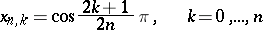
( are the roots of the Chebyshev polynomials), then in order that the interpolation process converges on the interval
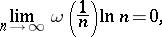
  it suffices that the following condition holds:
where  is the modulus of continuity (cf. Continuity, modulus of) of
  on
on  .
.
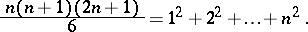
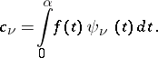
Another important problem in the calculus of finite differences is the problem of the summation of functions. Let  be a given function. It is required to find in finite form, exact or approximate, the sum
for fixed  ,
,  and large
  , when certain analytic properties of
  are known. In other words, the asymptotic behaviour of
  as
as  is studied. Let
  ,
,  (for simplicity) and suppose that a function
  can be found such that
 | (2) |
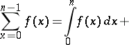
Then
 | (3) |
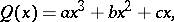
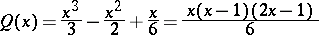
E.g., let  . The solution of (2) is sought in the form of a polynomial of degree three,
with undetermined coefficients. On substituting into equation (2) and equating coefficients of corresponding powers of  on the left-hand and right-hand sides, the polynomial has the form:
and
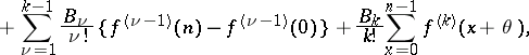
The solution to equation (2) cannot always be obtained in finite form. It is therefore useful to have approximate formulas for the  . Such a formula is the Euler–MacLaurin formula. If
  has
has  derivatives and
  is even, the Euler–MacLaurin formula can be written as
where  (in general
  depends on
  ), and the
  are the Bernoulli numbers. If
  is a polynomial of degree less than
  , the remainder term vanishes.
There is a similarity between the problems of the calculus of finite differences and those of differential and integral calculus. The operation of finding the difference corresponds to that of finding the derivative; the solution of equation (2), which, as an operation, is the inverse of finding the finite difference, corresponds to finding a primitive, that is, an indefinite integral. Formula (3) is a direct analogue of the Newton–Leibniz formula. This similarity emerges in considering finite-difference equations. By a finite-difference equation is meant a relation
where  is a given function and
  is the required function. If all the
  are expressed in terms of
  , then the finite-difference equation is written in the form
 | (4) |
Its solution with respect to  is:
is:
 | (5) |
For given initial values  one can successively find
  , etc. After solving (4) with respect to
  :
:
one can, by setting  , find
  , then
  , etc. Thus, from the equation in terms of the initial data one can find the values of
  at all the points
  , where
  is an integer. Consider, for
  the linear equation
 | (6) |
where  and
and  are given functions on the set
  . The general solution of the inhomogeneous equation (6) is the sum of a particular solution of the inhomogeneous equation and the general solution of the homogeneous equation
 | (7) |
If  are linearly independent solutions of (7), then the general solution of (7) is given by the formula
where  are arbitrary constants. The constants
  can be found by prescribing the initial conditions, that is, the values of
  . Linearly independent solutions
  (a fundamental system) are easily found in the case of an equation with constant coefficients:
 | (8) |
The solution of (8) is sought in the form  . The characteristic equation for
  is:
is:
Suppose that its roots  are all distinct. Then the system
  is a fundamental system of solutions of (8) and the general solution of (8) can be represented by the formula:
If  is a root of the characteristic equation of multiplicity
  , then the particular solutions corresponding to it are
  .
.
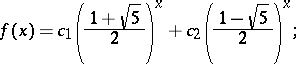
Suppose, for example, that one considers the sequence of numbers starting with 0 and 1 in which every successive number is equal to the sum of its two immediate predecessors: 0, 1, 1, 2, 3, 5, 8, 13 (the Fibonacci numbers). One seeks an expression for the general term of the sequence. Let
  ,
,  be the general term of the sequence; the conditions
form a difference equation with given initial conditions. The characteristic equation has the form  , its roots being
  ,
,  . Therefore
 and
and  being found from the initial conditions.
Equation (4) can be found not only when  varies discretely, taking values
  but also when
  varies continuously. Let
  be arbitrarily defined in the half-open interval
  . From (5) one obtains
  by setting
  . If
. If  is continuously defined in
  , then
  may prove to be discontinuous in the closed interval
  . If one wishes to deal with continuous solutions,
  needs to be defined on
  in such a way that by virtue of (5) it proves to be continuous in
  . Knowledge of
  in
in  enables one to find from (5)
  for
for  , then for
  , etc.
More general than (8) is the equation
 | (9) |
Here  are not necessarily integers and are not necessarily commensurable relative to one another. Equation (9) has the particular solutions
where  is a root of the equation
This equation has an infinite number of roots  . Consequently, (9) has an infinite number of particular solutions
  ,
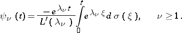
,  . Suppose that all the roots are simple. To express the solutions of (9) in terms of these elementary particular solutions, it is convenient to write the equation in the form:
 | (10) |
where  is a step function having jumps at the points
  , equal to
  , respectively. Let
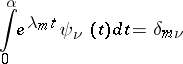
The functions  have the property:
( if
if  , and
, and  if
if  ), that is, they form a system that is bi-orthogonal to the system
  . On this basis, the solution
  of (10) corresponds to the series
 | (11) |
If (9) has the form
 | (12) |
(that is,  is a periodic function with period
  );
);  ; the roots of the equation
  are
are  (
( ); and (11) is the Fourier series of
  in complex form. The series (11) can be regarded as a generalization to the case of the difference equation (9) of the ordinary Fourier series corresponding to the simplest difference equation (12). Under certain conditions the series (11) converges to the solution
  . If
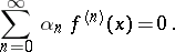
. If  is an analytic function, then (9) is expressible in the form of an equation of infinite order
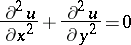
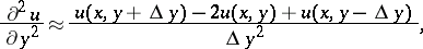
Differences of functions of several variables are introduced by analogy with differences of functions of one variable. For example, suppose that it is required to solve the problem of finding numerically the solution of the Laplace equation
in the rectangle  ,
,  , for given values of
  on the boundary of the rectangle. The rectangle is divided into small rectangular cells with sides
  ,
,  . The values of the solution are sought at the vertices of these cells. At the vertices that lie on the boundary of the original rectangle, the values of
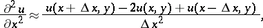
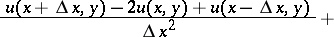
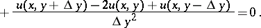
  are known. By applying the approximation (where second-order differences are in the numerators)
one obtains instead of the Laplace equation the following system of equations:
The point  runs through those vertices of cells that are situated in the interior of the original rectangle. Thus, a system of
  equations is constructed containing the same number of unknowns. By solving this algebraic system of equations, the values of
  at the vertices of the rectangles are obtained. When
  and
and  are small and the solution of the problem has a specified smoothness, the values so obtained are close to the exact values.
The calculus of finite differences was developed in parallel with that of the main branches of mathematical analysis. The calculus of finite differences first began to appear in works of P. Fermat, I. Barrow and G. Leibniz. In the 18th century it acquired the status of an independent mathematical discipline. The first systematic account of the calculus of finite differences was given by B. Taylor in 1715. The researches of mathematicians of the 19th century prepared the ground for the modern branches of the calculus of finite differences. The ideas and methods of the calculus of finite differences have been considerably developed in their application to analytic functions of a complex variable and to problems of numerical mathematics.
References
| [1] | A.A. Markov, "The calculus of finite differences" , Odessa (1910) (In Russian) |
| [2] | I.S. Berezin, N.P. Zhidkov, "Computing methods" , Pergamon (1973) (Translated from Russian) |
| [3] | A.O. [A.O. Gel'fond] Gelfond, "Differenzenrechnung" , Deutsch. Verlag Wissenschaft. (1958) (Translated from Russian) |
| [4] | N.S. Bakhvalov, "Numerical methods: analysis, algebra, ordinary differential equations" , MIR (1977) (Translated from Russian) |
See also Interpolation; Interpolation formula; Lagrange interpolation formula; Newton interpolation formula; Approximation of functions, linear methods.
References
| [a1] | L.M. Milne-Thomson, "The calculus of finite differences" , Macmillan (1933) Zbl 0008.01801; reprinted Dover (1981) Zbl 0477.39001 |
| [a2] | A.A. Samarskii, "Theorie der Differenzverfahren" , Akad. Verlagsgesell. Geest & Portig K.-D. (1984) (Translated from Russian) Zbl 0543.65067 |
| [a1] | Maurice V. Wilkes, "A short introduction to numerical analysis", Cambridge University Press (1966) ISBN 0-521-09412-7 Zbl 0149.10902
|