Hysteron

Only a very simple modification of the non-linearity "hysteron" is described below. See [a1] for the general definition and an identification theorem, that is, qualitative conditions under which a "black box" is a hysteron. Consider in the $ ( x,g ) $- plane the graphs of two continuous functions $ H _ {1} ( x ) $, $ H _ {2} ( x ) $ satisfying the inequality $ H _ {1} ( x ) < H _ {2} ( x ) $, $ x \in \mathbf R $. Suppose that the set $ \Omega = \{ {\{ x,g \} } : {x \in \mathbf R, H _ {1} ( x ) \leq g \leq H _ {2} ( x ) } \} $ is partitioned into the disjoint union of the continuous family of graphs of continuous functions $ g _ \alpha ( x ) $, where $ \alpha $ is a parameter. Each function $ g _ \alpha ( x ) $ is defined on its interval $ [ \eta _ \alpha ^ {1} , \eta _ \alpha ^ {2} ] $, $ \eta _ \alpha ^ {1} < \eta _ \alpha ^ {2} $, and $ g _ \alpha ( \eta _ \alpha ^ {1} ) = H _ {1} ( \eta _ \alpha ^ {1} ) $, $ g _ \alpha ( \eta _ \alpha ^ {2} ) = H _ {2} ( \eta _ \alpha ^ {2} ) $, that is, the end-points of the graphs of the functions $ g _ \alpha ( x ) $ belong to the union of the graphs of $ H _ {1} ( x ) $ and $ H _ {2} ( x ) $( 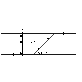see Fig.a2.).

Figure: h110430a

Figure: h110430b

Hysteron: Prandtl non-linearity

A hysteron is a transducer with internal states $ \xi $ from the segment $ [ 0,1 ] $ and with the following input–output operators. The variable output $ {\mathcal H} ( \xi _ {0} ) x ( t ) \equiv {\mathcal H} ( \xi _ {0} ,t _ {0} ) x ( t ) $( $ t \geq t _ {0} $) is defined by the formula

$$ {\mathcal H} ( \xi _ {0} ) x ( t ) = \left \{ \begin{array}{l} {g _ \alpha ( x ( t ) ) , \ \eta _ \alpha ^ {1} \leq x ( t ) \leq \eta _ \alpha ^ {2} , } \\ {H _ {1} ( x ( t ) ) , \ x ( t ) \leq \eta _ \alpha ^ {1} , } \\ {H _ {2} ( x ( t ) ) , \ \eta _ \alpha ^ {2} \leq x ( t ) , } \end{array} \right . $$

for monotone inputs $ x ( t ) $, $ t \geq t _ {0} $. The value of $ \alpha $ is determined by the initial state $ \xi $ to satisfy $ g _ \alpha ( x ( t _ {0} ) ) = \xi _ {0} H _ {1} ( x ( t _ {0} ) ) + ( 1 - \xi _ {0} ) H _ {2} ( x ( t _ {0} ) ) $ and the corresponding variable internal state is defined by

$$ \Xi ( \xi _ {0} ) x ( t ) = { \frac{ {\mathcal H} ( \xi _ {0} ) x ( t ) - H _ {1} ( x ( t ) ) }{H _ {2} ( x ( t ) ) - H _ {1} ( x ( t ) ) } } . $$

For piecewise-monotone continuous inputs the output is constructed by the semi-group identity. The input–output operators can then be extended to the totality of all continuous inputs by continuity (see [a1]). The operators $ {\mathcal H} ( \xi _ {0} ) x ( t ) $, $ \Xi ( \xi _ {0} ) x ( t ) $ are defined for each continuous input and each initial state. They are continuous as operators in the space of continuous functions with the uniform metric (cf. also Metric).

A hysteron is called a Prandtl non-linearity if $ H _ {1} ( x ) \equiv - h $, $ H _ {2} ( x ) \equiv h $; $ g _ \alpha = kx - \alpha $, $ \alpha - h \leq x \leq \alpha + h $, $ \alpha \in \mathbf R $. This non-linearity describes the Prandtl model of ideal plasticity with Young modulus $ k $ and elastic limits $ h $. The parallel connections of a finite numbers of such elements describe the Besseling model of elasto-plasticity and the continual counterpart describe the Ishlinskii model.

See also Hysteresis.

References

[a1]	M.A. Krasnosel'skii, A.V. Pokrovskii, "Systems with hysteresis" , Springer (1989) (In Russian)