Difference between revisions of "Butcher series"
m (→Definitions: adding svg images) |
m (→Definitions: details) |
||
| Line 37: | Line 37: | ||
==Definitions== | ==Definitions== | ||
| − | A tree is a connected acyclic graph (cf. also [[Graph|Graph]]). A rooted tree is a tree with a distinguished node, called the root (which is drawn at the bottom of the sample trees in the Table). Two rooted trees | + | A tree is a connected acyclic graph (cf. also [[Graph|Graph]]). A rooted tree is a tree with a distinguished node, called the root (which is drawn at the bottom of the sample trees in the Table). Two rooted trees $t$ |
| − | and $ | + | and $\widehat{t}$ |
| − | are isomorphic (i.e. | + | are isomorphic (''i.e.'' equivalent) if and only if there is a [[Bijection|bijection]] $\sigma $ |
| − | from the nodes of $ | + | from the nodes of $t$ to the nodes of $\widehat{t}$ |
| − | to the nodes of $ | + | such that $ \sigma $ maps the root of $ t $ |
| − | such that $ \sigma $ | ||
| − | maps the root of $ t $ | ||
to the root of $ {\widehat{t} } $ | to the root of $ {\widehat{t} } $ | ||
and any two nodes $ n _ {1} $ | and any two nodes $ n _ {1} $ | ||
| − | and $ n _ {2} $ | + | and $ n _ {2} $ are connected by an edge in $ t $ |
| − | are connected by an edge in $ t $ | ||
if and only if $ \sigma ( n _ {1} ) $ | if and only if $ \sigma ( n _ {1} ) $ | ||
and $ \sigma ( n _ {2} ) $ | and $ \sigma ( n _ {2} ) $ | ||
are connected by an edge in $ {\widehat{t} } $. | are connected by an edge in $ {\widehat{t} } $. | ||
| − | The following bracket notation for rooted trees is very useful. Let | + | The following bracket notation for rooted trees is very useful. Let $\bullet$ |
| − | + | be the tree with one node. For rooted trees $ t_{1} \dots t _ {m} $ | |
| − | be the | ||
with $ \rho ( t _ {i} ) \geq 1 $ | with $ \rho ( t _ {i} ) \geq 1 $ | ||
for $ i = 1 \dots m $, | for $ i = 1 \dots m $, | ||
| Line 63: | Line 59: | ||
of $ t $ | of $ t $ | ||
is isomorphic to $ t $. | is isomorphic to $ t $. | ||
| + | |||
The rooted trees with at most four nodes are displayed in the table below. | The rooted trees with at most four nodes are displayed in the table below. | ||
Revision as of 19:28, 15 March 2023
B-series
Let $ y : \mathbf R \rightarrow {\mathbf R ^ {d} } $ be an analytic function satisfying an ordinary differential equation $ y ^ \prime ( x ) = f ( y ( x ) ) $. A Butcher series for $ y $ is a series of the form
$$ B ( a,y ( x ) ) = \sum _ {t \in T } a ( t ) F ( t ) ( y ( x ) ) { \frac{h ^ {\rho ( t ) } }{\rho ( t ) ! } } , $$
where $ T $ is the set of rooted trees, $ a ( t ) \in \mathbf R $ is the coefficient for the series associated with the tree $ t $, $ F ( t ) ( y ( x ) ) \in \mathbf R ^ {d} $ is the elementary differential associated with the tree $ t $, $ h \in \mathbf R $ is a stepsize or $ x $- increment, and $ \rho ( t ) $, often called the order of the tree $ t $, is the number of nodes in the tree $ t $. All terms will be defined below. For a more thorough discussion of Butcher series, see [a1] or [a2].
Definitions
A tree is a connected acyclic graph (cf. also Graph). A rooted tree is a tree with a distinguished node, called the root (which is drawn at the bottom of the sample trees in the Table). Two rooted trees $t$ and $\widehat{t}$ are isomorphic (i.e. equivalent) if and only if there is a bijection $\sigma $ from the nodes of $t$ to the nodes of $\widehat{t}$ such that $ \sigma $ maps the root of $ t $ to the root of $ {\widehat{t} } $ and any two nodes $ n _ {1} $ and $ n _ {2} $ are connected by an edge in $ t $ if and only if $ \sigma ( n _ {1} ) $ and $ \sigma ( n _ {2} ) $ are connected by an edge in $ {\widehat{t} } $.
The following bracket notation for rooted trees is very useful. Let $\bullet$ be the tree with one node. For rooted trees $ t_{1} \dots t _ {m} $ with $ \rho ( t _ {i} ) \geq 1 $ for $ i = 1 \dots m $, let $ t = [ t _ {1} \dots t _ {m} ] $ be the rooted tree formed by connecting a new root to the roots of each of $ t _ {1} \dots t _ {m} $. Clearly, $ \rho ( t ) = 1 + \sum _ {i = 1 } ^ {m} \rho ( t _ {i} ) $ and any rooted tree formed by permuting the subtrees $ t _ {1} \dots t _ {m} $ of $ t $ is isomorphic to $ t $.
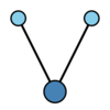
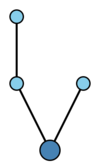
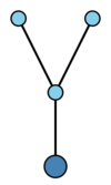
The rooted trees with at most four nodes are displayed in the table below.
<tbody> </tbody>
|
Using this bracket notation for rooted trees, one can recursively define elementary differentials, as follows. Let
$$ F ( \emptyset ) ( y ( x ) ) = y ( x ) , \quad F ( \bullet ) ( y ( x ) ) = f ( y ( x ) ) , $$
and, for $ t = [ t _ {1} \dots t _ {m} ] $ with $ \rho ( t _ {i} ) \geq 1 $ for $ i = 1 \dots m $,
$$ F ( t ) ( y ( x ) ) = $$
$$ = f ^ {( m ) } ( y ( x ) ) ( F ( t _ {1} ) ( y ( x ) ) \dots F ( t _ {m} ) ( y ( x ) ) ) , $$
where $ f ^ {( m ) } ( y ( x ) ) $, the $ m $ th derivative of $ f $ with respect to $ y $, is a multi-linear mapping.
Since $ y ( x ) $ satisfies $ y ^ \prime ( x ) = f ( y ( x ) ) $, it is not hard to show that
$$ y ^ {( i ) } ( x ) = \sum _ {t \in T _ {i} } \alpha ( t ) F ( t ) ( y ( x ) ) , $$
where $ y ^ {( i ) } ( x ) $ is the $ i $ th derivative of $ y $ with respect to $ x $, $ T _ {i} = \{ {t \in T } : {\rho ( t ) = i } \} $, and $ \alpha ( t ) $ is the number of distinct ways of labeling the nodes of $ t $ with the integers $ \{ 1 \dots \rho ( t ) \} $ such that the labels increase as you follow any path from the root to a leaf of $ t $. Consequently, one can write the Taylor series for $ y ( x ) $ as a Butcher series:
$$ \tag{a1 } y ( x + h ) = \sum _ {i = 0 } ^ \infty y ^ {( i ) } ( x ) { \frac{h ^ {i} }{i! } } = $$
$$ = \sum _ {t \in T } \alpha ( t ) F ( t ) ( y ( x ) ) { \frac{h ^ {\rho ( t ) } }{\rho ( t ) ! } } . $$
The importance of Butcher series stems from their use to derive and to analyze numerical methods for differential equations. For example, consider the $ s $- stage Runge–Kutta formula (cf. Runge–Kutta method)
$$ \tag{a2 } y _ {n + 1 } = y _ {n} + h \sum _ {i = 1 } ^ { s } b _ {i} k _ {i} , $$
$$ k _ {i} = f \left ( y _ {n} + h \sum _ {j = 1 } ^ { s } a _ {ij } k _ {j} \right ) , $$
for the ordinary differential equation $ y ^ \prime ( x ) = f ( y ( x ) ) $. Let $ b = ( b _ {1} \dots b _ {s} ) ^ {T} \in \mathbf R ^ {s} $ be the vector of weights and $ A = [ a _ {ij } ] \in \mathbf R ^ {s \times s } $ the coefficient matrix for (a2). Then it can be shown that $ y _ {n + 1 } $ can be written as the Butcher series
$$ \tag{a3 } y _ {n + 1 } = \sum _ {t \in T } \alpha ( t ) \psi ( t ) F ( t ) ( y _ {n} ) { \frac{h ^ {\rho ( t ) } }{\rho ( t ) ! } } , $$
where the coefficients $ \psi ( t ) \in \mathbf R $, defined below, depend only on the rooted tree $ t $ and the coefficients of the formula (a2).
To define $ \psi ( t ) $, first let
$$ \phi ( \emptyset ) = ( 1 \dots 1 ) ^ {T} \in \mathbf R ^ {s} , $$
$$ \phi ( \bullet ) = A \phi ( \emptyset ) , $$
and then, for $ t = [ t _ {1} \dots t _ {m} ] $ with $ \rho ( t _ {i} ) \geq 1 $ for $ i = 1 \dots m $, define $ \phi ( t ) $ recursively by
$$ \phi ( t ) = \rho ( t ) A ( \phi ( t _ {1} ) \dots \phi ( t _ {m} ) ) , $$
where the product of $ \phi $' s in the bracket is taken component-wise. Then
$$ \psi ( \emptyset ) = 1, $$
$$ \psi ( \bullet ) = \sum _ {i = 1 } ^ { s } b _ {i} , $$
and, for $ t = [ t _ {1} \dots t _ {m} ] $ with $ \rho ( t _ {i} ) \geq 1 $ for $ i = 1 \dots m $,
$$ \psi ( t ) = \rho ( t ) b ^ {T} ( \phi ( t _ {1} ) \dots \phi ( t _ {m} ) ) , $$
where, again, the product of $ \phi $' s in the bracket is taken componentwise.
Assuming that $ y ( x ) = y _ {n} $ and that $ \psi ( t ) = 1 $ for all trees $ t $ of order $ \leq p $, it follows immediately from (a1) and (a3) that
$$ y _ {n + 1 } = y ( x + h ) + {\mathcal O} ( h ^ {p + 1 } ) . $$
The order of (a2) is the largest such $ p $.
References
| [a1] | J.C. Butcher, "The numerical analysis of ordinary differential equations" , Wiley (1987) |
| [a2] | E. Hairer, S.P. Nørsett, G. Wanner, "Solving ordinary differential equations I: nonstiff problems" , Springer (1987) |
Butcher series. Encyclopedia of Mathematics. URL: http://encyclopediaofmath.org/index.php?title=Butcher_series&oldid=52562


