Difference between revisions of "Gregory formula"
(Importing text file) |
m (→Comments: links) |
||
| Line 27: | Line 27: | ||
====Comments==== | ====Comments==== | ||
| − | In [[#References|[1]]] above, the Gregory formulas are derived by means of the [[Fraser diagram|Fraser diagram]] and by integrating the resulting polynomial interpolation formula in each interval <img align="absmiddle" border="0" src="https://www.encyclopediaofmath.org/legacyimages/g/g045/g045120/g04512016.png" />. In this reference it is also observed that they can be derived from the [[Euler–MacLaurin formula|Euler–MacLaurin formula]] by suitable discretization of the "end corrections" . It turns out that this approach is rather straightforward and yields explicit expressions in terms of Stirling and Bernoulli numbers for the coefficients <img align="absmiddle" border="0" src="https://www.encyclopediaofmath.org/legacyimages/g/g045/g045120/g04512017.png" /> (cf. [[#References|[a2]]]). Yet another approach for deriving the Gregory formulas integrates the "initial-value problem" <img align="absmiddle" border="0" src="https://www.encyclopediaofmath.org/legacyimages/g/g045/g045120/g04512018.png" />, <img align="absmiddle" border="0" src="https://www.encyclopediaofmath.org/legacyimages/g/g045/g045120/g04512019.png" /> from <img align="absmiddle" border="0" src="https://www.encyclopediaofmath.org/legacyimages/g/g045/g045120/g04512020.png" /> until <img align="absmiddle" border="0" src="https://www.encyclopediaofmath.org/legacyimages/g/g045/g045120/g04512021.png" /> by a numerical integration method with step size <img align="absmiddle" border="0" src="https://www.encyclopediaofmath.org/legacyimages/g/g045/g045120/g04512022.png" />. Let <img align="absmiddle" border="0" src="https://www.encyclopediaofmath.org/legacyimages/g/g045/g045120/g04512023.png" /> denote the numerical approximation obtained for <img align="absmiddle" border="0" src="https://www.encyclopediaofmath.org/legacyimages/g/g045/g045120/g04512024.png" />. Since <img align="absmiddle" border="0" src="https://www.encyclopediaofmath.org/legacyimages/g/g045/g045120/g04512025.png" /> equals the integration of the function <img align="absmiddle" border="0" src="https://www.encyclopediaofmath.org/legacyimages/g/g045/g045120/g04512026.png" /> over the interval <img align="absmiddle" border="0" src="https://www.encyclopediaofmath.org/legacyimages/g/g045/g045120/g04512027.png" />, one may consider <img align="absmiddle" border="0" src="https://www.encyclopediaofmath.org/legacyimages/g/g045/g045120/g04512028.png" /> as an approximation integration of (or quadrature formula for) the function <img align="absmiddle" border="0" src="https://www.encyclopediaofmath.org/legacyimages/g/g045/g045120/g04512029.png" /> over the interval <img align="absmiddle" border="0" src="https://www.encyclopediaofmath.org/legacyimages/g/g045/g045120/g04512030.png" />. If the numerical integration method used for integrating <img align="absmiddle" border="0" src="https://www.encyclopediaofmath.org/legacyimages/g/g045/g045120/g04512031.png" />, <img align="absmiddle" border="0" src="https://www.encyclopediaofmath.org/legacyimages/g/g045/g045120/g04512032.png" /> is a linear multi-step method generated by polynomials <img align="absmiddle" border="0" src="https://www.encyclopediaofmath.org/legacyimages/g/g045/g045120/g04512033.png" /> and <img align="absmiddle" border="0" src="https://www.encyclopediaofmath.org/legacyimages/g/g045/g045120/g04512034.png" />, then the quadrature formula determined by <img align="absmiddle" border="0" src="https://www.encyclopediaofmath.org/legacyimages/g/g045/g045120/g04512035.png" /> is called a <img align="absmiddle" border="0" src="https://www.encyclopediaofmath.org/legacyimages/g/g045/g045120/g04512037.png" />-reducible quadrature formula. If the linear multi-step method <img align="absmiddle" border="0" src="https://www.encyclopediaofmath.org/legacyimages/g/g045/g045120/g04512038.png" /> is an Adams–Moulton method (cf. [[Adams method|Adams method]]) with starting values derived from interpolatory quadrature formulas, then <img align="absmiddle" border="0" src="https://www.encyclopediaofmath.org/legacyimages/g/g045/g045120/g04512039.png" /> is identical with a Gregory formula. The notion of <img align="absmiddle" border="0" src="https://www.encyclopediaofmath.org/legacyimages/g/g045/g045120/g04512040.png" />-reducible quadrature formulas was introduced by J. Matthys [[#References|[a4]]]. The general theory of these formulas is due to P.H.M. Wolkenfelt [[#References|[a6]]]. The particular case of the Gregory formulas is discussed in [[#References|[a5]]] and [[#References|[a2]]], and, especially, in [[#References|[a1]]]. These references give expressions for the residual term (or quadrature error) of Gregory formulas with differences of arbitrary orders. Gregory formulas play an important role in the numerical solution of Volterra equations (cf. [[#References|[a5]]], [[#References|[a3]]] and [[#References|[a2]]]). | + | In [[#References|[1]]] above, the Gregory formulas are derived by means of the [[Fraser diagram|Fraser diagram]] and by integrating the resulting polynomial interpolation formula in each interval <img align="absmiddle" border="0" src="https://www.encyclopediaofmath.org/legacyimages/g/g045/g045120/g04512016.png" />. In this reference it is also observed that they can be derived from the [[Euler–MacLaurin formula|Euler–MacLaurin formula]] by suitable discretization of the "end corrections" . It turns out that this approach is rather straightforward and yields explicit expressions in terms of [[Stirling numbers]] and [[Bernoulli numbers]] for the coefficients <img align="absmiddle" border="0" src="https://www.encyclopediaofmath.org/legacyimages/g/g045/g045120/g04512017.png" /> (cf. [[#References|[a2]]]). Yet another approach for deriving the Gregory formulas integrates the "initial-value problem" <img align="absmiddle" border="0" src="https://www.encyclopediaofmath.org/legacyimages/g/g045/g045120/g04512018.png" />, <img align="absmiddle" border="0" src="https://www.encyclopediaofmath.org/legacyimages/g/g045/g045120/g04512019.png" /> from <img align="absmiddle" border="0" src="https://www.encyclopediaofmath.org/legacyimages/g/g045/g045120/g04512020.png" /> until <img align="absmiddle" border="0" src="https://www.encyclopediaofmath.org/legacyimages/g/g045/g045120/g04512021.png" /> by a numerical integration method with step size <img align="absmiddle" border="0" src="https://www.encyclopediaofmath.org/legacyimages/g/g045/g045120/g04512022.png" />. Let <img align="absmiddle" border="0" src="https://www.encyclopediaofmath.org/legacyimages/g/g045/g045120/g04512023.png" /> denote the numerical approximation obtained for <img align="absmiddle" border="0" src="https://www.encyclopediaofmath.org/legacyimages/g/g045/g045120/g04512024.png" />. Since <img align="absmiddle" border="0" src="https://www.encyclopediaofmath.org/legacyimages/g/g045/g045120/g04512025.png" /> equals the integration of the function <img align="absmiddle" border="0" src="https://www.encyclopediaofmath.org/legacyimages/g/g045/g045120/g04512026.png" /> over the interval <img align="absmiddle" border="0" src="https://www.encyclopediaofmath.org/legacyimages/g/g045/g045120/g04512027.png" />, one may consider <img align="absmiddle" border="0" src="https://www.encyclopediaofmath.org/legacyimages/g/g045/g045120/g04512028.png" /> as an approximation integration of (or quadrature formula for) the function <img align="absmiddle" border="0" src="https://www.encyclopediaofmath.org/legacyimages/g/g045/g045120/g04512029.png" /> over the interval <img align="absmiddle" border="0" src="https://www.encyclopediaofmath.org/legacyimages/g/g045/g045120/g04512030.png" />. If the numerical integration method used for integrating <img align="absmiddle" border="0" src="https://www.encyclopediaofmath.org/legacyimages/g/g045/g045120/g04512031.png" />, <img align="absmiddle" border="0" src="https://www.encyclopediaofmath.org/legacyimages/g/g045/g045120/g04512032.png" /> is a linear multi-step method generated by polynomials <img align="absmiddle" border="0" src="https://www.encyclopediaofmath.org/legacyimages/g/g045/g045120/g04512033.png" /> and <img align="absmiddle" border="0" src="https://www.encyclopediaofmath.org/legacyimages/g/g045/g045120/g04512034.png" />, then the quadrature formula determined by <img align="absmiddle" border="0" src="https://www.encyclopediaofmath.org/legacyimages/g/g045/g045120/g04512035.png" /> is called a <img align="absmiddle" border="0" src="https://www.encyclopediaofmath.org/legacyimages/g/g045/g045120/g04512037.png" />-reducible quadrature formula. If the linear multi-step method <img align="absmiddle" border="0" src="https://www.encyclopediaofmath.org/legacyimages/g/g045/g045120/g04512038.png" /> is an Adams–Moulton method (cf. [[Adams method|Adams method]]) with starting values derived from interpolatory quadrature formulas, then <img align="absmiddle" border="0" src="https://www.encyclopediaofmath.org/legacyimages/g/g045/g045120/g04512039.png" /> is identical with a Gregory formula. The notion of <img align="absmiddle" border="0" src="https://www.encyclopediaofmath.org/legacyimages/g/g045/g045120/g04512040.png" />-reducible quadrature formulas was introduced by J. Matthys [[#References|[a4]]]. The general theory of these formulas is due to P.H.M. Wolkenfelt [[#References|[a6]]]. The particular case of the Gregory formulas is discussed in [[#References|[a5]]] and [[#References|[a2]]], and, especially, in [[#References|[a1]]]. These references give expressions for the residual term (or quadrature error) of Gregory formulas with differences of arbitrary orders. Gregory formulas play an important role in the numerical solution of Volterra equations (cf. [[#References|[a5]]], [[#References|[a3]]] and [[#References|[a2]]]). |
====References==== | ====References==== | ||
<table><TR><TD valign="top">[a1]</TD> <TD valign="top"> H. Brass, "Quadraturverfahren" , Vandenhoeck & Ruprecht (1977)</TD></TR><TR><TD valign="top">[a2]</TD> <TD valign="top"> H. Brunner, P.J. van der Houwen, "The numerical solution of Volterra equations" , North-Holland (1986)</TD></TR><TR><TD valign="top">[a3]</TD> <TD valign="top"> H. Brunner, J.D. Lambert, "Stability of numerical methods for Volterra integro-differential equations" ''Computing'' , '''12''' (1974) pp. 75–89</TD></TR><TR><TD valign="top">[a4]</TD> <TD valign="top"> J. Matthys, "A stable linear multistep method for Volterra integro-differential equations" ''Numer. Math.'' , '''27''' (1976) pp. 85–94</TD></TR><TR><TD valign="top">[a5]</TD> <TD valign="top"> J. Steinberg, "Numerical solution of Volterra integral equations" ''Numer. Math.'' , '''19''' (1972) pp. 212–217</TD></TR><TR><TD valign="top">[a6]</TD> <TD valign="top"> P.H.M. Wolkenfelt, "The construction of reducible quadrature rules for Volterra integral and integro-differential equations" ''IMA J. Numer. Anal.'' , '''2''' (1982) pp. 131–152</TD></TR></table> | <table><TR><TD valign="top">[a1]</TD> <TD valign="top"> H. Brass, "Quadraturverfahren" , Vandenhoeck & Ruprecht (1977)</TD></TR><TR><TD valign="top">[a2]</TD> <TD valign="top"> H. Brunner, P.J. van der Houwen, "The numerical solution of Volterra equations" , North-Holland (1986)</TD></TR><TR><TD valign="top">[a3]</TD> <TD valign="top"> H. Brunner, J.D. Lambert, "Stability of numerical methods for Volterra integro-differential equations" ''Computing'' , '''12''' (1974) pp. 75–89</TD></TR><TR><TD valign="top">[a4]</TD> <TD valign="top"> J. Matthys, "A stable linear multistep method for Volterra integro-differential equations" ''Numer. Math.'' , '''27''' (1976) pp. 85–94</TD></TR><TR><TD valign="top">[a5]</TD> <TD valign="top"> J. Steinberg, "Numerical solution of Volterra integral equations" ''Numer. Math.'' , '''19''' (1972) pp. 212–217</TD></TR><TR><TD valign="top">[a6]</TD> <TD valign="top"> P.H.M. Wolkenfelt, "The construction of reducible quadrature rules for Volterra integral and integro-differential equations" ''IMA J. Numer. Anal.'' , '''2''' (1982) pp. 131–152</TD></TR></table> | ||
Revision as of 19:11, 21 November 2014
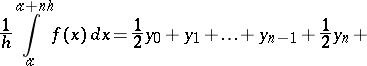
for the approximate integration of a function 
The formula
 |
 |
 |
where 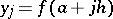 , and
, and  are the differences of the function
  of order
  at the points
  ,
,  and
and
 |
In particular,
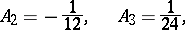 |
 |
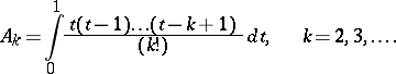
Gregory's formula is obtained by the integration of the interpolation polynomial with nodes at  . Gregory's formula with differences of orders up to
  inclusive can be obtained from the Newton–Cotes quadrature formula of closed type (cf. Cotes formulas), and for this reason the residual terms of the two formulas are identical. The simplest variant of Gregory's formula was proposed by J. Gregory in 1668.
References
| [1] | I.S. Berezin, N.P. Zhidkov, "Computing methods" , Pergamon (1973) (Translated from Russian) |
Comments
In [1] above, the Gregory formulas are derived by means of the Fraser diagram and by integrating the resulting polynomial interpolation formula in each interval  . In this reference it is also observed that they can be derived from the Euler–MacLaurin formula by suitable discretization of the "end corrections" . It turns out that this approach is rather straightforward and yields explicit expressions in terms of Stirling numbers and Bernoulli numbers for the coefficients
  (cf. [a2]). Yet another approach for deriving the Gregory formulas integrates the "initial-value problem"
  ,
,  from
from  until
until  by a numerical integration method with step size
  . Let
. Let  denote the numerical approximation obtained for
  . Since
  equals the integration of the function
  over the interval
  , one may consider
  as an approximation integration of (or quadrature formula for) the function
  over the interval
  . If the numerical integration method used for integrating
  ,
,  is a linear multi-step method generated by polynomials
  and
and  , then the quadrature formula determined by
  is called a
  -reducible quadrature formula. If the linear multi-step method
  is an Adams–Moulton method (cf. Adams method) with starting values derived from interpolatory quadrature formulas, then
  is identical with a Gregory formula. The notion of
  -reducible quadrature formulas was introduced by J. Matthys [a4]. The general theory of these formulas is due to P.H.M. Wolkenfelt [a6]. The particular case of the Gregory formulas is discussed in [a5] and [a2], and, especially, in [a1]. These references give expressions for the residual term (or quadrature error) of Gregory formulas with differences of arbitrary orders. Gregory formulas play an important role in the numerical solution of Volterra equations (cf. [a5], [a3] and [a2]).
References
| [a1] | H. Brass, "Quadraturverfahren" , Vandenhoeck & Ruprecht (1977) |
| [a2] | H. Brunner, P.J. van der Houwen, "The numerical solution of Volterra equations" , North-Holland (1986) |
| [a3] | H. Brunner, J.D. Lambert, "Stability of numerical methods for Volterra integro-differential equations" Computing , 12 (1974) pp. 75–89 |
| [a4] | J. Matthys, "A stable linear multistep method for Volterra integro-differential equations" Numer. Math. , 27 (1976) pp. 85–94 |
| [a5] | J. Steinberg, "Numerical solution of Volterra integral equations" Numer. Math. , 19 (1972) pp. 212–217 |
| [a6] | P.H.M. Wolkenfelt, "The construction of reducible quadrature rules for Volterra integral and integro-differential equations" IMA J. Numer. Anal. , 2 (1982) pp. 131–152 |
Gregory formula. Encyclopedia of Mathematics. URL: http://encyclopediaofmath.org/index.php?title=Gregory_formula&oldid=34712