Non-precise data

Real data obtained from measurement processes are not precise numbers or vectors but are more or less non-precise. This uncertainty is different from measurement errors and has to be described formally in order to obtain realistic results by mathematical models.

A real-life example is the water level of a river at a fixed time. It is typically not a precise multiple of the scale unit for height measurements. This water level is a fuzzy quantity called non-precise. In the past this kind of uncertainty was neglected in describing such data. The reason for that is the idea of the existence of a "true" water level which is identified with a real number times the measurement unit. But this is not realistic. The formal description of such non-precise water levels can be given using the intensity of the wetness of the gauge to obtain the so-called characterizing functions (see below).

Further examples of non-precise data are readings on digital measurement equipments, readings of pointers on scales, colour intensity pictures and light points on screens.

Non-precise data are different from measurement errors because in error models the observed values $y _ { i }$ are considered to be numbers, i.e. $y _ { i } = x _ { i } + \epsilon _ { i }$, where $\epsilon_{i}$ denotes the error of the $i$th observation (cf. also Numerical analysis).

Historically, non-precise data were not studied sufficiently. Some earlier work was done in interval arithmetic. In general, non-precise sets in the form of fuzzy sets were considered by L.A. Zadeh. Some publications combining fuzzy imprecision and stochastic uncertainty came up in the 1980s, see [a2]. Some of these approaches are more theoretically oriented. An applicable approach for statistical analysis of non-precise data is given in [a4].

Characterizing functions of non-precise numbers.

In the case of measurements of one-dimensional quantities, non-precise observations can be reasonably described by so-called fuzzy numbers $x ^ { * }$. Fuzzy numbers are generalizations of real numbers in the following sense.

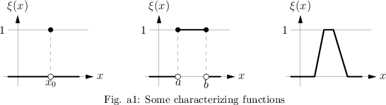
Each real number $X \in \mathbf R$ is characterized by its indicator function $I_{ \{ x \} } ( \cdot )$. Specializing the membership functions from fuzzy set theory, a fuzzy number is characterized by its so-called characterizing function $\xi ( . )$, which is a generalization of an indicator function. A characterizing function is a real-valued function of a real variable obeying the following:

1) $\xi : \mathbf{R} \rightarrow [ 0,1 ]$;

2) $\exists x \in \mathbf R $ such that $\xi ( x ) = 1$;

3) $\forall \alpha \in ( 0,1 ]$, the so-called $\alpha$-cut $B _ { \alpha } = \{ x \in \mathbf{R} : \xi ( x ) \geq \alpha \}$ is a closed finite interval. Characterizing functions describe the imprecision of a single observation. They should not be confused with probability densities, which describe the stochastic variation of a random quantity $X$ (cf. also Probability distribution). Examples of characterizing functions are depicted in Fig.a1.

A fundamental problem is how to obtain the characterizing function of a non-precise observation. This depends on the area of application. An example is as follows.

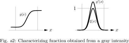
For data in the form of gray intensities in one dimension, as boundaries of regions the gray intensity $g ( x )$ as an increasing function of one real variable $x$ can be used to obtain the characterizing function $\xi ( x )$ in the following way. Take the derivative $( d / d x ) g ( x )$ and divide it by its maximum. The resulting function, or its convex hull, can be used as characterizing function of the non-precise observation.

In Fig.a2 the construction of the characterizing function from a gray intensity is explained.

Non-precise samples.

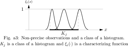
Taking observations of a one-dimensional continuous quantity $X$ in order to estimate the distribution of $X$, usually a finite sequence $x _ { 1 } ^ { * } , \ldots , x _ { n } ^ { * }$ of non-precise numbers is obtained. These non-precise data are given in form of $n$ characterizing functions $\xi _ { 1 } ( . ) , \ldots , \xi _ { n } ( . )$ corresponding to $x _ { 1 } ^ { * } , \ldots , x _ { n } ^ { * }$. Facing this kind of samples, even a most simple concept like the histogram has to be modified. This is necessary because, for a given class $K_j$ in a histogram, for a non-precise observation $x _ { i } ^ {\color{blue} *}$ with characterizing function $\xi _ { i }(.)$ obeying $\xi _ { i } ( x ) > 0$ for an element $x \in K_j $ and $\xi _ { i } ( y ) > 0$ for an element $y \in K _ { j } ^ { c }$, it is not possible to decide whether or not $x _ { i } ^ {\color{blue} *}$ is an element of $K_j$. The situation is explained in Fig.a3.

A generalization of the concept of histogram is possible by defining so-called fuzzy histograms. For such histograms the height of the histogram over a fixed class $K_j$ is a fuzzy number $h _ { j } ^ { * }$. For the definition of the characterizing function of $h _ { j } ^ { * }$, see [a3]. For other concepts of statistics in the case of non-precise data, see [a4].

Non-precise vectors.

In the case of multi-variate data $\underline { x } = ( x _ { 1 } , \dots , x _ { n } )$, for example the position of an object on a radar screen, the observations are non-precise vectors $\underline{x} ^ { * }$. Such non-precise vectors are characterized by so-called vector-characterizing functions $\xi _ { \underline{x}^{*}} ( . , \dots , . )$. These vector-characterizing functions $\xi _ { \underline{x}^{*}} ( . , \dots , . )$ are real-valued functions of $n$ real variables $x _ { 1 } , \ldots , x _ { n }$ obeying the following:

a) $\xi _ { \underline{x}^*} : \mathbf{R} ^ { n } \rightarrow [ 0,1 ]$;

b) $\exists \underline{x} = ( x _ { 1 } , \dots , x _ { n } ) \in \mathbf{R} ^ { n }$ such that ;

c) $\forall \alpha \in ( 0,1 ]$, the $\alpha$-cut $B _ { \alpha } ( \underline{x} ^ { * } ) = \{ \underline{x} \in \mathbf{R} ^ { n } : \xi _ { \underline{x} ^ { * } } ( \underline{x} ) \geq \alpha \}$ is a closed and star-shaped subset with finite $n$-dimensional content.

Functions of non-precise arguments.

For the generalization of functions of real variables, the so-called extension principle from fuzzy set theory is used. This principle generalizes a function to the situation when the value of the argument variable is non-precise.

Let $\psi : \mathbf{R} ^ { n } \rightarrow \mathbf{R}$ be a classical real-valued function of $n$ variables. If the argument $\underline { x } = ( x _ { 1 } , \dots , x _ { n } )$ is precise, then the value $\psi ( \underline{x} )$ of the function is also a precise real number. For a non-precise argument $\underline{x} ^ { * }$ it is natural that the value $\psi ( \underline{x} ^ { * } )$ becomes non-precise also. The quantitative description of this imprecision is done by using the characterizing function $\eta ( . )$ of $\psi ( \underline{x} ^ { * } )$. Let $\xi ( ., \dots , . )$ be the vector-characterizing function of the fuzzy vector $\underline{x} ^ { * }$. Then, for all real numbers $y$, the values $\eta ( y )$, are given by the extension principle in the following way:

\begin{equation*} \eta ( y ) = \left\{ \begin{array} { l l } { \operatorname { sup } \{ \xi ( \underline{x} ) : \underline{x} \in {\bf R} ^ { n } , \psi ( \underline{x} ) = y \} , } & { \psi ^ { - 1 } ( y ) \neq \emptyset ,} \\ { 0 , } & { \psi ^ { - 1 } ( y ) = \emptyset .} \end{array} \right. \end{equation*}

For continuous functions $\psi ( . )$ it can be proved that $\eta ( . )$ is a characterizing function, see [a4].

Non-precise functions.

Consider the monitoring of quantities in continuous time for real measurements. The results are functions of time with non-precise values. Therefore the concept of a non-precise function is necessary. These are functions whose values are fuzzy numbers. Let $M$ be the domain of the non-precise function $f ^ { * } ( . )$ and let be the set of all fuzzy numbers; then

\begin{equation*} f ^ { * } : M \rightarrow \mathcal{F} ( \mathbf{R} ). \end{equation*}

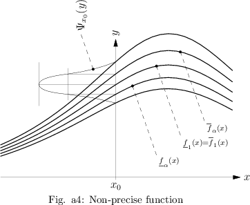
A non-precise function can also be considered as a family of fuzzy numbers with characterizing functions $\psi _ { x } ( \cdot )$, i.e.

\begin{equation*} \{ \psi _ { x } ( . ) \widehat{=} f ^ { * } ( x ) : x \in M \}. \end{equation*}

A graphical description of non-precise functions can be given using the $\alpha$-cuts $\left[ \underline { f } \square _ { \alpha } ( x ) , \overline { f } _ { \alpha } ( x ) \right]$ of the fuzzy numbers $f ^ { * } ( x )$.

The curves $x \rightarrow \underline { f } \square_{\alpha} ( x )$ and $x \rightarrow \overline { f } _ { \alpha } ( x )$ are called lower and upper $\alpha$-level curves. Taking a finite suitable number of $\alpha$-levels from $( 0,1 ]$ and depicting the corresponding $\alpha$-level curves in a diagram, a good graphical display of the non-precise function is obtained. An example is given in Fig.a4.

Applications.

Whenever measurements have to be modeled, non-precise numbers appear. This occurs in the initial conditions for differential equations, in the time-dependent description of quantities, as well as in statistical inference.

Mathematical methods for the analysis of non-precise data exist and should be used in order to obtain more realistic results from mathematical modeling.

References

[a1]	"Modelling uncertain data" H. Bandemer (ed.) , Akad. Berlin (1993)
[a2]	"Combining fuzzy imprecision with probabilistic uncertainty in decision making" J. Kacprzyk (ed.) M. Fedrizzi (ed.) , Lecture Notes Economics and Math. Systems , 310 , Springer (1988)
[a3]	R. Viertl, "Statistics with non-precise data" J. Comput. Inform. Techn. , 4 : 4 (1996)
[a4]	R. Viertl, "Statistical methods for non-precise data" , CRC (1996)