Non-linear stability of numerical methods
Numerical stability theory for the initial value problem $y ^ { \prime } = f ( x , y )$, $y ( 0 ) = y _ { 0 }$, where $f : \mathbf{R} \times \mathbf{C} ^ { n } \rightarrow \mathbf{C} ^ { n }$, is concerned with the question of whether the numerical discretization inherits the dynamic properties of the differential equation. Stability concepts are usually based on structural assumptions on $f$. For non-linear problems, the breakthrough was achieved by G. Dahlquist in his seminal paper [a3]. There, he studied multi-step discretizations of problems satisfying a one-sided Lipschitz condition. Let $\langle \, .\, ,\, . \, \rangle$ denote an inner product on $\mathbf{C} ^ { n }$ and let $\| .\|$ be the induced norm.
Runge–Kutta methods.
An $s$-stage Runge–Kutta discretization of $y ^ { \prime } = f ( x , y )$, $y ( 0 ) = y _ { 0 }$ is given by
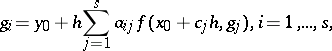 |
\begin{equation*} y _ { 1 } = y _ { 0 } + h \sum _ { i = 1 } ^ { s } b _ { i }\, f ( x _ { 0 } + c _ { i } h , g _ { i } ). \end{equation*}
Here, $h$ denotes the step-size and $y_1$ is the Runge–Kutta approximation to $y ( x _ { 0 } + h )$. (For a thorough discussion of such methods, see [a1], [a2], and [a4]; see also Runge–Kutta method.)
B-stability.
If the problem satisfies the global contractivity condition
\begin{equation*} \operatorname { Re } \langle f ( x , y ) - f ( x , z ) , y - z \rangle \leq 0 , y , z \in \mathbf{C} ^ { n }, \end{equation*}
then the difference of two solutions is a non-increasing function of $x$. Let $y_1$, $z_1$ denote the numerical solutions after one step of size $h$ with initial values $y _ { 0 }$, $z_0$, respectively. A Runge–Kutta method is called B-stable (or sometimes BN-stable), if the contractivity condition implies $\| y _ { 1 } - z _ { 1 } \| \leq \| y _ { 0 } - z _ { 0 } \|$ for all $h > 0$. Examples of B-stable Runge–Kutta methods are given below. The definition of B-stability extends to arbitrary one-step methods in an obvious way.
Algebraic stability.
A Runge–Kutta method is called algebraically stable if its coefficients satisfy
i) $b _ { i } \geq 0$, $i = 1 , \dots , s$;
ii) $( b _ { i } a _ { i j } + b _ { j } a _ { j i } - b _ { i } b _ { j } ) _ { i , j = 1 } ^ { s }$ is positive semi-definite. Algebraic stability plays an important role in the theory of B-convergence. Note that algebraic stability implies B-stability. For non-confluent methods, i.e. $c _ { i } \neq c _ { j }$ for $i \neq j$, both concepts are equivalent. The following families of implicit Runge–Kutta methods are algebraically stable and therefore B-stable: Gauss, RadauIA, RadauIIA, LobattoIIIC.
Error growth function.
Let $\mathcal{F} _ { \nu }$ ($\nu \in \mathbf{R}$) denote the class of all problems satisfying the one-sided Lipschitz condition
\begin{equation*} \operatorname { Re } \langle f ( x , y ) - f ( x , z ) , y - z \rangle \leq \nu \| y - z \| ^ { 2 } , y , z \in \mathbf{C} ^ { n }. \end{equation*}
For $\nu > 0$, this condition is weaker than contractivity and allows trajectories to expand with increasing $x$. For any given real number $\xi $ and step-size $h > 0$, set $\nu = \xi / h$ and denote by $\varphi ( \xi )$ the smallest number for which the estimate $\| y _ { 1 } - z _ { 1 } \| \leq \varphi ( \xi ) \| y _ { 0 } - z _ { 0 } \|$ holds for all problems in $\mathcal{F} _ { \nu }$. The function $\varphi$ is called error growth function. For B-stable Runge–Kutta methods, the error growth function is superexponential, i.e. satisfies $\varphi ( 0 ) = 1$ and $\varphi ( \xi _ { 1 } ) \varphi ( \xi _ { 2 } ) \leq \varphi ( \xi _ { 1 } + \xi _ { 2 } )$ for all $\xi _ { 1 }$, $\xi_2$ having the same sign. This result can be used in the asymptotic stability analysis of Runge–Kutta methods, see [a5].
Linear multi-step methods.
A linear multi-step discretization of $y ^ { \prime } = f ( x , y )$ is given by
\begin{equation*} \sum _ { i = 0 } ^ { k } \alpha _ { i } y _ { m + i } = h \sum _ { i = 0 } ^ { k } \beta _ { i } \,f ( x _ { m + i} , y _ { m + i } ). \end{equation*}
Let $\rho ( \zeta ) = \sum _ { i = 0 } ^ { k } \alpha _ { i } \zeta ^ { i }$ and $\sigma ( \zeta ) = \sum _ { i = 0 } ^ { k } \beta _ { i } \zeta ^ { i }$ be the generating polynomials. Using the normalization $\sigma ( 1 ) = 1$, the associated one-leg method is defined by
\begin{equation*} \sum _ { i = 0 } ^ { k } \alpha _ { i } y _ { m + i } = h f \left( \sum _ { i = 0 } ^ { k } \beta _ { i } x _ { m + i } , \sum _ { i = 0 } ^ { k } \beta _ { i } y _ { m + i } \right). \end{equation*}
(For a thorough discussion, see [a4].) A one-leg method is called G-stable if there exists a real symmetric positive-definite $k$-dimensional matrix $G$ such that any two numerical solutions satisfy $\| Y _ { 1 } - Z _ { 1 } \| _ { G } \leq \| Y _ { 0 } - Z _ { 0 } \| _ { G }$ for all step-sizes $h > 0$, whenever the problem is contractive ($\nu = 0$). Here, $Y _ { m } = ( y _ { m + k - 1} , \ldots , y _ { m } ) ^ { T }$ and
\begin{equation*} \| Y _ { m } \| _ { G } ^ { 2 } = \sum _ { i , j = 1 } ^ { k } g_{ij} \langle y _ { m + i - 1} , y _ { m + j - 1} \rangle. \end{equation*}
G-stability is closely related to linear stability: If the generating polynomials have no common divisor, then the multi-step method is A-stable if and only if the corresponding one-leg method is G-stable. Thus, the $2$-step BDF method is G-stable. There is also a purely algebraic condition that implies G-stability.
The concepts of G-stability and algebraic stability have been successfully extended to general linear methods, see [a1] and [a4].
Notwithstanding the merits of B- and G-stability, contractive problems have quite simple dynamics. Other classes of problems have been considered that admit a more complex behaviour. For a review, see [a7].
The long-time behaviour of time discretizations of non-linear evolution equations is an active field of research at the moment (1998). Basically, two different approaches exist for the analysis of numerical stability:
a) energy estimates;
b) estimates for the linear problem, combined with perturbation techniques. Whereas energy estimates require algebraic stability on the part of the methods, linear stability (A($\theta$)-stability) is sufficient for the second approach. (For an illustration of these techniques in connection with convergence, see [a6].) Both approaches offer their merits. The latter, however, is in particular important for methods that are not B-stable, e.g., for linearly implicit Runge–Kutta methods.
References
| [a1] | J. Butcher, "The numerical analysis of ordinary differential equations: Runge–Kutta and general linear methods" , Wiley (1987) |
| [a2] | K. Dekker, J.G. Verwer, "Stability of Runge–Kutta methods for stiff nonlinear differential equations" , North-Holland (1984) |
| [a3] | G. Dahlquist, "Error analysis for a class of methods for stiff non-linear initial value problems" , Numerical Analysis, Dundee 1975 , Lecture Notes Math. , 506 , Springer (1976) pp. 60–72 |
| [a4] | E. Hairer, G. Wanner, "Solving ordinary differential equations II: Stiff and differential-algebraic problems" , Springer (1996) (Edition: Second, revised) |
| [a5] | E. Hairer, M. Zennaro, "On error growth functions of Runge–Kutta methods" Appl. Numer. Math. , 22 (1996) pp. 205–216 |
| [a6] | Ch. Lubich, A. Ostermann, "Runge–Kutta approximations of quasi-linear parabolic equations" Math. Comp. , 64 (1995) pp. 601–627 |
| [a7] | A. Stuart, A.R. Humphries, "Model problems in numerical stability theory for initial value problems" SIAM Review , 36 (1994) pp. 226–257 |
Non-linear stability of numerical methods. Encyclopedia of Mathematics. URL: http://encyclopediaofmath.org/index.php?title=Non-linear_stability_of_numerical_methods&oldid=50652