Crank-Nicolson method
One of the most popular methods for the numerical integration (cf. Integration, numerical) of diffusion problems, introduced by J. Crank and P. Nicolson [a1] in 1947. They considered an implicit finite difference scheme to approximate the solution of a non-linear differential system of the type which arises in problems of heat flow.
In order to illustrate the main properties of the Crank–Nicolson method, consider the following initial-boundary value problem for the heat equation
\begin{equation*} \left\{ \begin{array} { l } { u _ { t } - u _ { x x } = 0 , \quad 0 < x < 1,0 < t, } \\ { u ( 0 , t ) = u ( 1 , t ) = 0 , \quad 0 < t, } \\ { u ( x , 0 ) = u ^ { 0 } ( x ) , \quad 0 \leq x \leq 1. } \end{array} \right. \end{equation*}
To approximate the solution $u$ of this model problem on $[ 0,1 ] \times [ 0 , T ]$, one introduces the grid
\begin{equation*} \{ ( x _ { j } , t _ { n } ) : x _ { j } = j h , t _ { n } = n k , 0 \leq j \leq J , 0 \leq n \leq N \}, \end{equation*}
where $J$ and $N$ are positive integers, and $h = 1 / J$ and $k = T / N$ are the step sizes in space and time, respectively. One looks for approximations $U _ { j } ^ { n }$ to $u _ { j } ^ { n } = u ( x _ { j } , t _ { n } )$, and to this end one replaces derivatives by finite-difference formulas. Setting $\delta ^ { 2 } U _ { j } = h ^ { - 2 } ( U _ { j + 1 } - 2 U _ { j } + U _ { j - 1 } )$, then the Crank–Nicolson method for the considered problem takes the form
\begin{equation*} \frac { U _ { j } ^ { n + 1 } - U _ { j } ^ { n } } { k } = \delta ^ { 2 } \left( \frac { U _ { j } ^ { n + 1 } + U _ { j } ^ { n } } { 2 } \right), \end{equation*}
$1 \leq j \leq J - 1$, $0 \leq n \leq N - 1$, with boundary conditions
\begin{equation*} U _ { 0 } ^ { n } = U _ { J } ^ { n } = 0 , \quad 1 \leq n \leq N, \end{equation*}
and numerical initial condition
\begin{equation*} U ^ { 0 } j = P _ { j } , \quad 0 \leq j \leq J, \end{equation*}
where $P_{j}$ is an approximation to $u ^ { 0 } ( x_j )$. Note that each term in the difference equation can be interpreted as an approximation to the corresponding one in the differential equation at $( x_{j} , ( n + 1 / 2 ) k )$.
Whenever the theoretical solution $u$ is sufficiently smooth, it can be proved, by Taylor series expansions that there exists a positive constant $C$, which depends only on $u$ and $T$, such that the truncation error
\begin{equation*} \tau _ { j } ^ { n + 1 } = \frac { u _ { j } ^ { n + 1 } - u _ { j } ^ { n } } { k } - \delta ^ { 2 } \left( \frac { u _ { j } ^ { n + 1 } + u _ { j } ^ { n } } { 2 } \right) \end{equation*}
satisfies
\begin{equation*} | \tau _ { j } ^ { n + 1 } | \leq C ( h ^ { 2 } + k ^ { 2 } ), \end{equation*}
$1 \leq j \leq J - 1$, $0 \leq n \leq N - 1$. Thus, the Crank–Nicolson scheme is consistent of second order both in time and space.
The stability study ([a2], [a3]) in the discrete $l_2$-norm can be made by Fourier analysis or by the energy method. One introduces the discrete operator
\begin{equation*} ( \mathcal{L} _ { h k } V ) _ { j } ^ { n + 1 } = \frac { V _ { j } ^ { n + 1 } - V _ { j } ^ { n } } { k } - \delta ^ { 2 } \left( \frac { V _ { j } ^ { n + 1 } + V _ { j } ^ { n } } { 2 } \right), \end{equation*}
$1 \leq j \leq J - 1$, $0 \leq n \leq N - 1$, where it is assumed that $V _ { 0 } ^ { n } = V _ { j } ^ { n } = 0$; and sets $\| \mathbf{V} \| ^ { 2 } = \sum _ { j = 1 } ^ { J - 1 } h | V _ { j } | ^ { 2 }$. There exists a positive constant $C$, which is independent of $h$ and $k$, such that
\begin{equation*} \| \mathbf{V} ^ { n } \| ^ { 2 } \leq \| \mathbf{V} ^ { 0 } \| ^ { 2 } + C \sum _ { m = 1 } ^ { n } k \| ( \mathcal{L} _ { h k } V ) ^ { m } \| ^ { 2 } , \end{equation*}
$1 \leq n$. The stability estimate holds without any restriction on the step sizes $h$ and $k$; thus, the Crank–Nicolson method is said to be unconditionally stable. Convergence is derived by consistency and stability and, as $h \rightarrow 0$ and $k \rightarrow 0$, one finds
\begin{equation*} \| \mathbf{U }^ { n } - \mathbf{u} ^ { n } \| \leq \| \mathbf{U} ^ { 0 } - \mathbf{u} ^ { 0 } \| + O ( h ^ { 2 } + k ^ { 2 } ), \end{equation*}
$1 \leq n \leq N$. Stability can also be established in the discrete $H ^ { 1 }$-norm by means of an energy argument [a3]. Denoting $\Delta V _ { j } = h ^ { - 1 } ( V _ { j } - V _ { j - 1 } )$, and $\| \Delta \mathbf{V} \| ^ { 2 } = \sum _ { j = 1 } ^ { J } h | \Delta V _ { j } | ^ { 2 }$, where $V _ { 0 } = V _ { J } = 0$, then the following stability estimate holds:
\begin{equation*} \| \Delta \mathbf{V} ^ { n } \| ^ { 2 } \leq \| \Delta \mathbf{V} ^ { 0 } \| ^ { 2 } + \sum _ { m = 1 } ^ { n } k \| ( \mathcal{L} _ { h k } V ) ^ { m } \| ^ { 2 } , \end{equation*}
$1 \leq n$. Therefore, if the theoretical solution $u$ is sufficiently smooth, then
\begin{equation*} \| \Delta ( \mathbf{U} ^ { n } - \mathbf{u} ^ { n } ) \| \leq \| \Delta ( \mathbf{U} ^ { 0 } - \mathbf{u} ^ { 0 } ) \| + O ( h ^ { 2 } + k ^ { 2 } ), \end{equation*}
$1 \leq n \leq N$. Note that the above inequality implies a convergence estimate in the maximum norm.
An important question is to establish a maximum principle for the approximations obtained with the Crank–Nicolson method, similar to the one satisfied by the solutions of the heat equation. Related topics are monotonicity properties and, in particular, the non-negativity (or non-positivity) of the numerical approximations. Maximum-principle and monotonicity arguments can be used to derive convergence in the $l_ { \infty }$-norm. It can be proved ([a2], [a3]) that a choice of the step sizes such that $k h ^ { - 2 } \leq 1$ and the condition
\begin{equation*} ( \mathcal{L} _ { h k } V ) _ { j } ^ { n + 1 } \leq 0,\;1 \leq j \leq J - 1,\;0 \leq n \leq N - 1, \end{equation*}
imply
\begin{equation*} V _ { j } ^ { n } \leq \operatorname { max } \left( \operatorname { max } _ { 0 \leq j \leq J } V _ { j } ^ { 0 } , \operatorname { max } _ { 0 \leq m \leq n } V _ { 0 } ^ { m } , \operatorname { max } _ { 0 \leq m \leq n } V _ { j } ^ { m } \right), \end{equation*}
$0 \leq i \leq J$, $0 \leq n \leq N$. Note that if $( \mathcal{L} _ { h k } U ) _ { j } ^ { n } \equiv 0$ and $U _ { 0 } ^ { n } = U _ { J } ^ { n } = 0$, then the following stability estimate in the maximum norm holds:
\begin{equation*} \| \mathbf{U} ^ { n } \| _ { \infty } \leq C \| \mathbf{U} ^ { 0 } \| _ { \infty } , 1 \leq n, \end{equation*}
where $C = 1$ and $\| \mathbf{U} ^ { n } \| _ { \infty } = \operatorname { max } _ { 1 \leq j \leq J } | U _ { j } ^ { n } |$. This estimate is still valid with $C = 1$ if $k h ^ { - 2 } \leq 3 / 2$ (see [a4]), and also it holds without any restriction between the step sizes but then a value $C > 1$ has to be accepted in the bound ([a3], [a5]).
From a computational point of view, the Crank–Nicolson method involves a tridiagonal linear system to be solved at each time step. This can be carried out efficiently by Gaussian elimination techniques [a2]. Because of that and its accuracy and stability properties, the Crank–Nicolson method is a competitive algorithm for the numerical solution of one-dimensional problems for the heat equation.
The Crank–Nicolson method can be used for multi-dimensional problems as well. For example, in the integration of an homogeneous Dirichlet problem in a rectangle for the heat equation, the scheme is still unconditionally stable and second-order accurate. Also, the system to be solved at each time step has a large and sparse matrix, but it does not have a tridiagonal form, so it is usually solved by iterative methods. The amount of work required to solve such a system is sufficiently large, so other numerical schemes are also taken into account here, such as alternating-direction implicit methods [a6] or fractional-steps methods [a7]. On the other hand, it should be noted that, for multi-dimensional problems in general domains, the finite-element method is better suited for the spatial discretization than the finite-difference method is.
The Crank–Nicolson method can be considered for the numerical solution of a wide variety of time-dependent partial differential equations. Consider the abstract Cauchy problem
\begin{equation*} u _ { t } = \mathcal{F} ( t , u ) , 0 < t , u ( x , 0 ) = u ^ { 0 } ( x ), \end{equation*}
where $\mathcal{F}$ represents a partial differential operator (cf. also Differential equation, partial; Differential operator) which differentiates the unknown function $u$ with respect to the space variable $x$ in its space domain in $\mathbf{R} ^ { p }$, and $u$ may be a vector function. In the numerical integration of such problem, one can distinguish two stages: space discretization and time integration.
For the spatial discretization one can use finite differences, finite elements, spectral techniques, etc., and then a system of ordinary differential equations is obtained, which can be written as
\begin{equation*} \frac { d } { d t } U _ { h } = F _ { h } ( t , U _ { h } ) , 0 < t , U _ { h } ( 0 ) = u ^ { 0_h } , \end{equation*}
where $h$ is the space discretization parameter (the spatial grid size of a finite-difference or finite-element scheme, the inverse of the highest frequency of a spectral scheme, etc.) and $u _ { h } ^ { 0 }$ is a suitable approximation to the theoretical initial condition $u ^ { 0 }$.
The phrase "Crank–Nicolson method" is used to express that the time integration is carried out in a particular way. However, there is no agreement in the literature as to what time integrator is called the Crank–Nicolson method, and the phrase sometimes means the trapezoidal rule [a8] or the implicit midpoint method [a6]. Let $k$ be the time step and introduce the discrete time levels $t _ { n } = n k $, $n \geq 0$. If one uses the trapezoidal rule, then the full discrete method takes the form
\begin{equation*} \frac { U _ { h } ^ { n + 1 } - U _ { h } ^ { n } } { k } = \frac { 1 } { 2 } F _ { h } ( t _ { n } , U _ { h } ^ { n } ) + \frac { 1 } { 2 } F _ { h } ( t _ { n +1 } , U _ { h } ^ { n + 1 } ), \end{equation*}
while when the implicit midpoint method is considered, one obtains
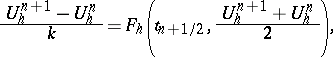 |
where $t _ { n+1/2 } = t _ { n } + k / 2$, and $U _ { h } ^ { n }$ is the approximation to $U _ { h } ( t _ { n } )$. Both methods coincide for linear autonomous problems, but they are different in general. For instance, the midpoint rule is symplectic [a9], while the trapezoidal rule does not satisfy this property.
The Crank–Nicolson method applied to several problems can be found in [a8], [a10], [a11], [a12], [a13] and [a14].
References
| [a1] | J. Crank, P. Nicolson, "A practical method for numerical evaluation of solutions of partial differential equations of the heat-conduction type" Proc. Cambridge Philos. Soc. , 43 (1947) pp. 50–67 |
| [a2] | K.W. Morton, D.F. Mayers, "Numerical solution of partial differential equations" , Cambridge Univ. Press (1994) |
| [a3] | V. Thomee, "Finite difference methods for linear parabolic equations" P.G. Ciarlet (ed.) J.L. Lions (ed.) , Handbook of Numerical Analysis , 1 , Elsevier (1990) pp. 9–196 |
| [a4] | J.F.B.M. Kraaijevanger, "Maximum norm contractivity of discretization schemes for the heat equation" Appl. Numer. Math. , 9 (1992) pp. 475–496 |
| [a5] | C. Palencia, "A stability result for sectorial operators in Banach spaces" SIAM J. Numer. Anal. , 30 (1993) pp. 1373–1384 |
| [a6] | A.R. Mitchell, D.F. Griffiths, "The finite difference method in partial differential equations" , Wiley (1980) |
| [a7] | N.N. Yanenko, "The method of fractional steps" , Springer (1971) |
| [a8] | J.G. Verwer, J.M. Sanz-Serna, "Convergence of method of lines approximations to partial differential equations" Computing , 33 (1984) pp. 297–313 |
| [a9] | J.M. Sanz-Serna, M.P. Calvo, "Numerical Hamiltonian problems" , Chapman&Hall (1994) |
| [a10] | Y. Tourigny, "Optimal $H ^ { 1 }$ estimates for two time-discrete Galerkin approximations of a nonlinear Schroedinger equation" IMA J. Numer. Anal. , 11 (1991) pp. 509–523 |
| [a11] | G.D. Akrivis, "Finite difference discretization of the Kuramoto–Sivashinsky equation" Numer. Math. , 63 (1992) pp. 1–11 |
| [a12] | S.K. Chung, S.N. Ha, "Finite element Galerkin solutions for the Rosenau equation" Appl. Anal. , 54 (1994) pp. 39–56 |
| [a13] | I.M. Kuria, P.E. Raad, "An implicit multidomain spectral collocation method for stiff highly nonlinear fluid dynamics problems" Comput. Meth. Appl. Mech. Eng. , 120 (1995) pp. 163–182 |
| [a14] | G. Fairweather, J.C. Lopez-Marcos, "Galerkin methods for a semilinear parabolic problem with nonlocal boundary conditions" Adv. Comput. Math. , 6 (1996) pp. 243–262 |
Crank-Nicolson method. Encyclopedia of Mathematics. URL: http://encyclopediaofmath.org/index.php?title=Crank-Nicolson_method&oldid=55358