Spherical matrix distribution

A random matrix $X ( p \times n )$ (cf. also Matrix variate distribution) is said to have

a right spherical distribution if $X : = X \Lambda$ for all $\Lambda \in \mathcal{O} ( n )$;

a left spherical distribution if $X := \Gamma X$ for all $\Gamma \in \mathcal{O} ( p )$; and

a spherical distribution if $X := \Gamma X \Lambda$ for all $\Gamma \in \mathcal{O} ( p )$ and all $\Lambda \in \mathcal{O} ( n )$. Here, $\mathcal{O} ( r )$ denotes the class of orthogonal $( r \times r )$-matrices (cf. also Orthogonal matrix).

Instead of saying that $X ( p \times n )$ "has a" (left, right) spherical distribution, one also says that $X ( p \times n )$ itself is (left, right) spherical.

If $X ( p \times n )$ is right spherical, then

a) its transpose $X ^ { \prime }$ is left spherical;

b) $- X$ is right spherical, i.e. $- X := X$; and

c) for $T ( p \times n )$, its characteristic function is of the form $\phi ( T T ^ { \prime } )$.

The fact that $X ( p \times n )$ is right (left) spherical with characteristic function $\phi ( T T ^ { \prime } )$, is denoted by $X \sim \operatorname { RS } _ { p , n } ( \phi )$ (respectively, $X \sim \operatorname { LS } _ { p , n } ( \phi )$).

Let $X \sim \operatorname { RS } _ { p , n } ( \phi )$. Then:

1) for a constant matrix $A ( q \times p )$, $A X \sim \operatorname { RS } _ { q , n } ( \psi )$, where $\psi ( T T ^ { \prime } ) = \phi ( A ^ { \prime } T T ^ { \prime } A )$, $T ( q \times n )$;

2) for $X = ( X _ { 1 } , X _ { 2 } )$, where $X _ { 1 }$ is a $( p \times m )$-matrix, $X _ { 1 } \sim \operatorname { RS } _ { p , m } ( \phi )$;

3) if $X X ^ { \prime } = I _ { p }$, $p \leq n$, then $X \sim \mathcal{U} _ { p , n}$, the uniform distribution on the Stiefel manifold $\mathcal{O} ( p , n ) = \{ H ( p \times n ) : H H ^ { \prime } = I _ { p } \}$.

The probability distribution of a right spherical matrix $X ( p \times n )$ is fully determined by that of $X X ^ { \prime }$. It follows that the uniform distribution is the unique right spherical distribution over $\mathcal{O} ( p , n )$. For a right spherical matrix the density need not exist in general. However, if $X$ has a density with respect to Lebesgue measure on , then it is of the form $f ( X X ^ { \prime } )$.

Examples of spherical distributions with a density.

When $X \sim N _ { p , n } ( 0 , \Sigma \otimes I _ { n } )$, the density of $X$ is

$$\begin{equation*} \frac { 1 } { ( 2 \pi ) ^ { n p / 2 } } | \Sigma | ^ { - n / 2 } \operatorname { etr } \left\{ - \frac { 1 } { 2 } \Sigma ^ { - 1 } X X ^ { \prime } \right\} , X \in \mathbf{R} ^ { p \times n }, \end{equation*}$$

with characteristic function

$$\begin{equation*} \operatorname { etr } \left\{ - \frac { 1 } { 2 } \Sigma ^ { - 1 } T T ^ { \prime } \right\}. \end{equation*}$$

Here, is the exponential trace function:

$$\begin{equation*} \operatorname { etr } ( A ) = \operatorname { exp } ( \operatorname { tr } ( A ) ). \end{equation*}$$

When $X \sim T _ { p , n } ( \delta , 0 , \Sigma , I _ { n } )$, the density of $X$ is

$$\begin{equation*} \frac { \Gamma _ { p } \left[ \frac { \delta + n + p - 1 } { 2 } \right] } { ( 2 \pi ) ^ { n p / 2 } | \Sigma | ^ { n / 2 } \Gamma _ { p } \left[ \frac { \delta + p - 1 } { 2 } \right] }. \end{equation*}$$

$$\begin{equation*} .\left| I _ { p } + \Sigma ^ { - 1 } X X ^ { \prime } \right| ^ { - ( \delta + n + p - 1 ) / 2 } , X \in \mathbf{R} ^ { p \times n }, \end{equation*}$$

with characteristic function

$$\begin{equation*} \frac { B _ { - ( \delta + p - 1 ) / 2} \left( \frac { 1 } { 4 } \Sigma T T ^ { \prime } \right) } { \Gamma _ { p } \left[ \frac { 1 } { 2 } ( \delta + p - 1 ) \right] }, \end{equation*}$$

where $B _ { \delta } ( \cdot )$ is Herz's Bessel function of the second kind and of order $\delta$.

If $X ( p \times n )$ is right spherical and $K ( n \times m )$ is a fixed matrix, then the distribution of $X K$ depends on $K$ only through $K ^ { \prime } K$. Now, if $K ^ { \prime } K = I _ { m }$, then the distribution of $X K$ is right spherical.

Let $X = ( X _ { 1 } , X _ { 2 } )$, with $X _ { 1 } ( p \times ( n - m ) )$, $X _ { 2 } ( p \times m )$, and let $K ^ { \prime } = ( K _ { 1 } ^ { \prime } , K _ { 2 } ^ { \prime } )$, where $K _ { 1 } ( ( n - m ) \times m ) = 0$, $K _ { 2 } ( m \times m ) = I _ { m }$. Then $K ^ { \prime } K = I _ { m }$, and therefore $X K = X _ { 2 }$ is right spherical.

If the distribution of $X$ is a mixture of right spherical distributions, then $X$ is right spherical. It follows that if $X ( p \times n )$, conditional on a random variable $v$, is right spherical and $Q ( q \times p )$ is a function of $v$, then $Q X$ is right spherical.

The results given above have obvious analogues for left spherical distributions.

Stochastic representation of spherical distributions.

Let $X \sim \operatorname { RS } _ { p , n } ( \phi )$. Then there exists a random matrix $A ( p \times p )$ such that

$$\begin{equation} \tag{a1} X : = A U, \end{equation}$$

where $U \sim \mathcal{U} _ { p , n }$ is independent of $A$.

The matrix $A$ in the stochastic representation (a1) is not unique. One can take it to be a lower (upper) triangular matrix with non-negative diagonal elements or a right spherical matrix with $A \geq 0$. Further, if it is additionally assumed that $\mathsf P ( | XX ^ { \prime } | = 0 ) = 0$, then the distribution of $A$ is unique.

Given the assumption that $A$ is lower triangular in the above representation, one can prove that it is unique. Indeed, let $X \sim \operatorname { RS } _ { p , n } ( \phi )$ and $\mathsf{P} ( | XX ^ { \prime } | \neq 0 ) = 1$. Then for $A$, $B$ lower triangular matrices with positive diagonal elements and $U \sim \mathcal{U} _ { p , n }$, $Q \sim \mathcal{U} _ { p , n }$:

i) $X : = A U$ and $X = B U \Rightarrow A : = B$;

ii) $X : = A U$ and $X : = A Q \Rightarrow U : = Q$.

For studying the spherical distribution, singular value decomposition of the matrix $X ( p \times n )$ provides a powerful tool. When $p \leq n$, let $X = G \Lambda H$, where $G \in \mathcal{O} ( p )$, $H \in \mathcal{O} ( p , n )$, $\Lambda = \operatorname { diag } ( \lambda _ { 1 } , \dots , \lambda _ { p } )$, $\lambda _ { 1 } \geq \ldots \geq \lambda _ { p } \geq 0$, and the $\lambda _ { i }$ are the eigenvalues of $( X X ^ { \prime } ) ^ { 1 / 2 }$.

If $X ( p \times n )$, $p \leq n$, is spherical, then

$$\begin{equation} \tag{a2} X : = U \Lambda V, \end{equation}$$

where $U \sim \mathcal U _ { p , p }$, $V \sim {\cal U} _ { p , n }$ and $\Lambda$ are mutually independent.

If $X ( p \times n )$ is spherical, then its characteristic function is of the form $\phi ( \lambda ( T T ^ { \prime } ) )$, where $T ( p \times n )$, $\lambda ( T T ^ { \prime } ) = \operatorname { diag } ( \tau _ { 1 } , \dots , \tau _ { 1 } )$, and $\tau _ { 1 } \geq \ldots \geq \tau _ { p } \geq 0$ are the eigenvalues of $TT'$.

From the above it follows that, if the density of a spherical matrix $X$ exists, then it is of the form $f ( \lambda ( X X ^ { \prime } ) )$.

Let $X \sim \operatorname { RS } _ { p , n } ( \phi )$. If the second-order moments of $X$ exist (cf. also Moment), then

i) $\mathsf{E} ( X ) = 0$;

ii) $\operatorname { cov } ( X ) = V \otimes I _ { n }$, where $V = \mathsf{E} ( {\bf x} _ { 1 } {\bf x} _ { 1 } ^ { \prime } )$, $X = ( \mathbf{x} _ { 1 } , \dots , \mathbf{x} _ { n } )$.

Let $X \sim \operatorname { RS } _ { p , n } ( \phi )$ with density $f ( X X ^ { \prime } )$. Then the density of $S = X X ^ { \prime }$, $n \geq p$, is

$$\begin{equation*} \frac { \pi ^ { n p / 2 } } { \Gamma _ { p } ( n / 2 ) } | S | ^ { ( n - p - 1 ) / 2 } f ( S ) , \quad S > 0. \end{equation*}$$

Let $X \sim \operatorname { RS } _ { p , n } ( \phi )$ with density $f ( X X ^ { \prime } )$. Partition $X$ as $X = ( X _ { 1 } , \dots , X _ { r } )$, $X _ { i } ( p \times n _ { i } )$, $n _ { i } \geq p$, $i = 1 , \ldots , r$, $\sum _ { i = 1 } ^ { r } n _ { i } = n$. Define $S _ { i } = X _ { i } X_i ^ { \prime }$, $i = 1 , \ldots , r$. Then $( S _ { 1 } , \dots , S _ { r } ) \sim L _ { r } ^ { ( 1 ) } ( f , n _ { 1 } / 2 , \dots , n _ { r } / 2 )$ with probability density function

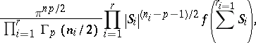$$\begin{equation*} S _ { i } > 0 , i = 1 , \dots , r. \end{equation*}$$

The above result has been generalized further. Let $X \sim \operatorname { RS } _ { p , n } ( \phi )$ with density $f ( X X ^ { \prime } )$, and let $A ( n \times n )$ be a symmetric matrix. Then

$$\begin{equation} \tag{a3} X A X ^ { \prime } \sim L _ { 1 } ^ { ( 1 ) } \left( f _ { 1 } , \frac { { k } } { 2 } \right), \end{equation}$$

where $f _ { 1 } ( T ) = W ^ { ( n - k ) / 2 } f ( T )$ is the Weyl fractional integral of order $( n - k ) / 2$ (cf. also Fractional integration and differentiation), if and only if $A ^ { 2 } = A$ and $\text{rank} ( A ) = k \geq p$. Further, let $A _ { 1 } ( n \times n ) , \dots , A _ { s } ( n \times n )$ be symmetric matrices. Then

$$\begin{equation} \tag{a4} \left( X A _ { 1 } X ^ { \prime } , \ldots , X A _ { s } X ^ { \prime } ) \sim L _ { s } ^ { ( 1 ) } ( f _ { 1 } , \frac { n _ { 1 } } { 2 } , \dots , \frac { n _ { s } } { 2 } \right), \end{equation}$$

where $f _ { 1 } ( T ) = W ^ { ( n - n _ { 1 } - \ldots - n _ { s } ) / 2 } f ( T )$, if and only if $A _ { i } A _ { j } = \delta _ { i j } A$, and $\operatorname{rank} ( A _ { i } ) = n_i$, $n _ { i } \geq p$, $i,j = 1 , \dots , s$.

References

[a1]	A.P. Dawid, "Spherical matrix distributions and multivariate model" J. R. Statist. Soc. Ser. B , 39 (1977) pp. 254–261
[a2]	K.T. Fang, Y.T. Zhang, "Generalized multivariate analysis" , Springer (1990)
[a3]	A.K. Gupta, T. Varga, "Elliptically contoured models in statistics" , Kluwer Acad. Publ. (1993)