|
|
| Line 1: |
Line 1: |
| − | $\def\l{\lambda}$
| + | ''of sets'' |
| − | A ''local dynamical system'' is a [[dynamical system]] (flow of a vector field, cascade of iterates of a self-map, or sometimes more involved construction) defined in an unspecifiedly small neighborhood of a fixed (rest) point. Application of local invertible self-map ("change of the variables") transforms a local dynamical system to an ''equivalent'' system. The local classification problem is to describe the equivalence classes of local dynamical systems, providing, if possible, the simplest or most convenient representative in each class.
| |
| | | | |
| − | ==Local dynamical systems and their equivalence==
| + | {{MSC|28C15}} |
| − | By a ''local'' [[dynamical system]] one usually understands one of the following:
| |
| − | * a (smooth, analytic, formal) vector field $v$ defined<ref>In the formal case instead of the germ we consider a tuple of formal Taylor series in the variables $x=(x_1,\dots,x_n)$.</ref> on a neighborhood $(\RR^n,0)$, $v:(\RR^n,0)\owns x\mapsto T_x(\RR^n,0)$, and vanishing at the origin, $v(0)=0$, or
| |
| − | *a (smooth, analytic, formal germ of a) invertible self-map $f\in\operatorname{Diff}(\RR^n,0)=\{$invertible maps of $(\RR^n,0)$ to itself fixing the origin, $f(0)=0\}$<ref>In the formal and analytic cases one can replace the real field $\RR$ by the field of complex numbers $\CC$.</ref>.
| |
| | | | |
| − | The "dynamical" idea is the possibility to iterate the self map, producing the cyclic group
| + | [[Category:Set functions and measures on topological spaces]] |
| − | $$
| |
| − | f^{\circ\ZZ}=\{\underbrace{f\circ \cdots\circ f}_{k\text{ times}}\,|\,k\in\ZZ\}\subseteq\operatorname{Diff}(\RR^n,0),
| |
| − | $$
| |
| − | or a one-parametric group<ref>As before, the "real time" $t\in\RR$ can be replaced by the "complex time" $t\in\CC$ given the appropriate context.</ref>
| |
| − | $$\exp \RR v=\{\exp tv\in\operatorname{Diff}(\RR^n,0)\,|\, t\in\RR,\ \exp[(t+s)v]=(\exp tv)\circ (\exp sv),\ \tfrac{\rd}{\rd t}|_{t=0}\exp tv=v\}
| |
| − | $$
| |
| − | with $v$ as the infinitesimal generator<ref>Note that all iterates (resp., flow maps) are defined only as ''germs'', thus the definition of the ''orbit'' $O(a)=\{f^{\circ k}(a)\}$ of a point $a\in(\RR^n,0)$ (forward, backward or bi-infinite) requires additional work.</ref>.
| |
| | | | |
| − | Two local dynamical systems of the same type are ''equivalent'', if there exists an invertible self-map $h\in\operatorname{Diff}(\RR^n,0)$ which conjugates them:
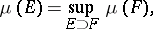
| + | A non-negative function <img align="absmiddle" border="0" src="https://www.encyclopediaofmath.org/legacyimages/b/b017/b017110/b0171101.png" /> of the subsets of a topological space <img align="absmiddle" border="0" src="https://www.encyclopediaofmath.org/legacyimages/b/b017/b017110/b0171102.png" /> possessing the following properties: 1) its domain of definition is the <img align="absmiddle" border="0" src="https://www.encyclopediaofmath.org/legacyimages/b/b017/b017110/b0171103.png" />-algebra <img align="absmiddle" border="0" src="https://www.encyclopediaofmath.org/legacyimages/b/b017/b017110/b0171104.png" /> of Borel sets (cf. [[Borel set|Borel set]]) in <img align="absmiddle" border="0" src="https://www.encyclopediaofmath.org/legacyimages/b/b017/b017110/b0171105.png" />, i.e. the smallest class of subsets in <img align="absmiddle" border="0" src="https://www.encyclopediaofmath.org/legacyimages/b/b017/b017110/b0171106.png" /> containing the open sets and closed with respect to the set-theoretic operations performed a countable number of times; and 2) <img align="absmiddle" border="0" src="https://www.encyclopediaofmath.org/legacyimages/b/b017/b017110/b0171107.png" /> if <img align="absmiddle" border="0" src="https://www.encyclopediaofmath.org/legacyimages/b/b017/b017110/b0171108.png" /> when <img align="absmiddle" border="0" src="https://www.encyclopediaofmath.org/legacyimages/b/b017/b017110/b0171109.png" />, i.e. <img align="absmiddle" border="0" src="https://www.encyclopediaofmath.org/legacyimages/b/b017/b017110/b01711010.png" /> is countably additive. A Borel measure <img align="absmiddle" border="0" src="https://www.encyclopediaofmath.org/legacyimages/b/b017/b017110/b01711011.png" /> is called regular if |
| − | $$
| |
| − | f\sim f'\iff\exists h:\ f\circ h=h\circ f',
| |
| − | \qquad\text{resp.,}\qquad
| |
| − | v\sim v'\iff\exists h:\ \rd h\cdot v=v'\circ h.
| |
| − | $$
| |
| − | Here $\rd h$ is the differential of $h$, acting on $v$ as a left multiplication by the Jacobian matrix $\bigl(\frac{\partial h}{\partial x}\bigr)$. Obviously, the equivalent systems have equivalent dynamics: if $h$ conjugates $f$ with $f'$, it also conjugates any iterate $f^{\circ k}$ with $f'^{\circ k}$, and conjugacy of vector fields implies that their flows are conjugated by $h$: $h\circ(\exp tv)=(\exp tv')\circ h$ for any $t\in\RR$.
| |
| | | | |
| − | A ''singularity'' (or ''singularity type'') of a local dynamical system is a subspace of germs defined by finitely many [[semialgebraic]] constraints on the initial Taylor coefficients of the germ. Examples:
| + | <table class="eq" style="width:100%;"> <tr><td valign="top" style="width:94%;text-align:center;"><img align="absmiddle" border="0" src="https://www.encyclopediaofmath.org/legacyimages/b/b017/b017110/b01711012.png" /></td> </tr></table> |
| − | * [[Hyperbolic dynamical system]]s: Self-maps tangent to linear automorphisms without modulus one eigenvalues, or vector fields whose linear part has no eigenvalues on the imaginary axis;
| |
| − | * [[Saddle node|Saddle-node]]s, self-maps having only one simple egenvalue $\mu=1$, resp., vector fields, whose linearization matrix has a simple eigenvalue $\lambda=0$;
| |
| − | * Cuspidal germs of vector fields on $(\RR^2,0)$ with the nilpotent linearization matrix $\bigl(\begin{smallmatrix}0&1\\0&0\end{smallmatrix}\bigr)$.
| |
| | | | |
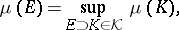
| − | The ''classification problem'' for a given singularity type requires to construct a list (finite or infinite, eventually involving parameters) of ''normal forms'', such that any local dynamical system of the given type is equivalent to one of these normal forms. | + | where <img align="absmiddle" border="0" src="https://www.encyclopediaofmath.org/legacyimages/b/b017/b017110/b01711013.png" /> belongs to the class <img align="absmiddle" border="0" src="https://www.encyclopediaofmath.org/legacyimages/b/b017/b017110/b01711014.png" /> of closed subsets in <img align="absmiddle" border="0" src="https://www.encyclopediaofmath.org/legacyimages/b/b017/b017110/b01711015.png" />. The study of Borel measures is often connected with that of Baire measures, which differ from Borel measures only in their domain of definition: They are defined on the smallest <img align="absmiddle" border="0" src="https://www.encyclopediaofmath.org/legacyimages/b/b017/b017110/b01711016.png" />-algebra <img align="absmiddle" border="0" src="https://www.encyclopediaofmath.org/legacyimages/b/b017/b017110/b01711017.png" /> with respect to which all continuous functions on <img align="absmiddle" border="0" src="https://www.encyclopediaofmath.org/legacyimages/b/b017/b017110/b01711018.png" /> are measurable. A Borel measure <img align="absmiddle" border="0" src="https://www.encyclopediaofmath.org/legacyimages/b/b017/b017110/b01711019.png" /> (or a Baire measure <img align="absmiddle" border="0" src="https://www.encyclopediaofmath.org/legacyimages/b/b017/b017110/b01711020.png" />) is said to be <img align="absmiddle" border="0" src="https://www.encyclopediaofmath.org/legacyimages/b/b017/b017110/b01711022.png" />-smooth if <img align="absmiddle" border="0" src="https://www.encyclopediaofmath.org/legacyimages/b/b017/b017110/b01711023.png" /> for any net <img align="absmiddle" border="0" src="https://www.encyclopediaofmath.org/legacyimages/b/b017/b017110/b01711024.png" /> of closed sets which satisfies the condition <img align="absmiddle" border="0" src="https://www.encyclopediaofmath.org/legacyimages/b/b017/b017110/b01711025.png" /> (or <img align="absmiddle" border="0" src="https://www.encyclopediaofmath.org/legacyimages/b/b017/b017110/b01711026.png" /> for any net <img align="absmiddle" border="0" src="https://www.encyclopediaofmath.org/legacyimages/b/b017/b017110/b01711027.png" /> of sets which are zero sets of continuous functions and such that <img align="absmiddle" border="0" src="https://www.encyclopediaofmath.org/legacyimages/b/b017/b017110/b01711028.png" />). A Borel measure <img align="absmiddle" border="0" src="https://www.encyclopediaofmath.org/legacyimages/b/b017/b017110/b01711029.png" /> (or Baire measure <img align="absmiddle" border="0" src="https://www.encyclopediaofmath.org/legacyimages/b/b017/b017110/b01711030.png" />) is said to be tight if |
| | | | |
| − | A particular case of classification problems is the study of ''linearizability''.
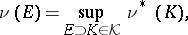
| + | <table class="eq" style="width:100%;"> <tr><td valign="top" style="width:94%;text-align:center;"><img align="absmiddle" border="0" src="https://www.encyclopediaofmath.org/legacyimages/b/b017/b017110/b01711031.png" /></td> </tr></table> |
| − | ;Definition | |
| − | A germ of a vector field with the Taylor expansion $v(x)=Ax+O(\|x\|^2)$ (resp., of a self-map with the Taylor expansion $f(x)=Mx+O(\|x\|^2)$ is ''linearizable'' (formally, smoothly or analytically), if it is conjugated to the linear vector field $v'(x)=Ax$, (resp., to the linear automorphism $f(x)=Mx$.
| |
| − | <small> | |
| − | ----
| |
| − | <references/> | |
| − | </small> | |
| | | | |
| − | ====Remarks==== | + | where <img align="absmiddle" border="0" src="https://www.encyclopediaofmath.org/legacyimages/b/b017/b017110/b01711032.png" /> is the class of compact subsets on <img align="absmiddle" border="0" src="https://www.encyclopediaofmath.org/legacyimages/b/b017/b017110/b01711033.png" /> (or |
| − | When speaking of local dynamics, one can also consder a slightly more general situation of arbitrary finitely generated group action on $\operatorname{Diff}(\RR^n,0)$ or $\operatorname{Diff}(\CC^n,0)$. For instance, one can consider ''commuting tuples of vector fields'' $\{v_1,\dots,v_k\}$ on $(\RR^n,0)$, $[v_i,v_j]=0$. This "dynamical system with $k$-dimensional time" corresponds to the action of the abelian group $\R^k$ on $(\R^n,0)$ and is important in the theory of [[integrable system]]s. Another, in a sense, completely opposite case, corresponds to the simultaneous classification of several self-maps $\{f_1,\dots,f_k\}\subseteq\operatorname{Diff}(\C^1,0)$. This problem defines (generically) the action of the free group $F_k$ on $k$ generators. Classification (to the extent is possible) of such tuples is important for understanding the complex topology of holomorphic foliations. In most such cases one does not have any finite lists of normal forms, thus the classification problems have to address some more general properties of the corresponding actions.
| |
| | | | |
| − | Besides vector fields, one can also consider a problem of local classification of [[Pfaffian form]]s. A Pfaffian (differential 1-)form $\xi$ on the real plane $(\R^2,0)$ defines an [[integrability|integrable]] distribution of lines (eventually with a singularity at the origin) $\{\xi=0\}$ of null spaces which is tangent to a suitable vector field $v_\xi$. If $\xi=A(x,y)\rd x+B(x,y)\rd y$ with, say, analytic germs $A,B$ having an isolated common root at the origin, then the vector field $v_\xi$ takes the form $\dot x=-B(x,y)$, $\dot y=A(x,y)$, which is also analytic. However, the distribution of null spaces is preserved if the 1-form $\xi$ is replaced by a form $u\cdot\xi$, where $u$ is the germ of a non-vanishing function. Classification of null distributions of Pfaffian 1-forms is often referred to as the ''orbital'' classification of the respective vector fields: two vector fields are orbitally equivalent if the foliations by integral curves, generated by these fields, are conjugate by a local diffeomorphism (smooth or analytic) of $(\R^n,0)$.
| + | <table class="eq" style="width:100%;"> <tr><td valign="top" style="width:94%;text-align:center;"><img align="absmiddle" border="0" src="https://www.encyclopediaofmath.org/legacyimages/b/b017/b017110/b01711034.png" /></td> </tr></table> |
| | | | |
| − | In higher dimension, however, the integrability of the 1-form $\xi$ has to be explicitly postulated; the classification problem for such forms (modulo a scalar multiple, as before) is equivalent to classification of codimension one foliations near a singular point.
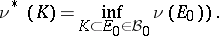
| + | where |
| | | | |
| − | ===Analytic, formal and smooth equivalence=== | + | <table class="eq" style="width:100%;"> <tr><td valign="top" style="width:94%;text-align:center;"><img align="absmiddle" border="0" src="https://www.encyclopediaofmath.org/legacyimages/b/b017/b017110/b01711035.png" /></td> </tr></table> |
| − | Technically, the local classification problem for dynamical systems is no different from the for [[Normal form (for singularities)|left-right classification problem for germs of smooth maps]]. In particular, one would assume looking for conjugacy $h$ in the same regularity class as the objects of classification (formal conjugacy for formal germs, smooth conjugacy for smooth germs, analytic conjugacy for analytic germs). This approach usually works for the left-right equivalence (to the extent where a meaningful classification exists).
| |
| | | | |
| − | However, for local dynamical systems a completely new phenomenon of divergence arises: very often a given analytic local dynamical system admits a relatively simple formal normal form (i.e, is formally equivalent to a simple, say, polynomial or even linear germ), yet the formal series for the conjugacy diverges and the analytic classification turns out to be immensely more delicate.
| + | Tightness and <img align="absmiddle" border="0" src="https://www.encyclopediaofmath.org/legacyimages/b/b017/b017110/b01711036.png" />-smoothness are restrictions which ensure additional smoothness of measures, and which in fact often hold. Under certain conditions Baire measures can be extended to Borel measures. For instance, if <img align="absmiddle" border="0" src="https://www.encyclopediaofmath.org/legacyimages/b/b017/b017110/b01711037.png" /> is a completely-regular Hausdorff space, then any <img align="absmiddle" border="0" src="https://www.encyclopediaofmath.org/legacyimages/b/b017/b017110/b01711038.png" />-smooth (tight) finite Baire measure can be extended to a regular <img align="absmiddle" border="0" src="https://www.encyclopediaofmath.org/legacyimages/b/b017/b017110/b01711039.png" />-smooth (tight) finite Borel measure. In the study of measures on locally compact spaces Borel measures (or Baire measures) is the name sometimes given to measures defined on the <img align="absmiddle" border="0" src="https://www.encyclopediaofmath.org/legacyimages/b/b017/b017110/b01711040.png" />-ring of sets generated by the compact (or <img align="absmiddle" border="0" src="https://www.encyclopediaofmath.org/legacyimages/b/b017/b017110/b01711041.png" />-compact) sets and which are finite on compact sets. Often, by the Borel measure on the real line one understands the measure defined on the Borel sets such that its value on an arbitrary segment is equal to the length of that segment. |
| | | | |
| − | ;Example
| + | ====References==== |
| − | A holomorphic self-map $f\in\operatorname{Diff}(\CC^1,0)$ tangent to the identity, i.e., of the form $f(z)=z+a_2z^2+a_3z^3+\cdots$ (the series converges, $a_2\ne0$) is formally equivalent to the cubic self-map $f'(z)=z+z^2+az^3$, with a formal invariant $a\in\CC$, yet the analytic classification of such self-maps has a ''functional invariant'', the so called [[Ecalle-Voronin modulus]], which shows that the same class of formal equivalence contains continuum of pairwise analytically non-equivalent self-maps distinguished by a certain auxiliary analytic function. The phenomenon is known today under the name of the [[Nonlinear Stokes phenomenon]], {{Cite|I93}}, {{Cite|IY}}.
| + | <table><TR><TD valign="top">[1]</TD> <TD valign="top"> V.S. Varadarajan, "Measures on topological spaces" ''Transl. Amer. Math. Soc. Ser. 2'' , '''48''' (1965) pp. 161–228 ''Mat. Sb.'' , '''55 (97)''' : 1 (1961) pp. 35–100 {{MR|0148838}} {{ZBL|}} </TD></TR><TR><TD valign="top">[2]</TD> <TD valign="top"> P.R. Halmos, "Measure theory" , v. Nostrand (1950) {{MR|0033869}} {{ZBL|0040.16802}} </TD></TR><TR><TD valign="top">[3]</TD> <TD valign="top"> J. Neveu, "Bases mathématiques du calcul des probabilités" , Masson (1970) {{MR|0272004}} {{ZBL|0203.49901}} </TD></TR></table> |
| | | | |
| − |
| |
| − | The $C^\infty$-smooth classification of smooth local dynamical systems occupies an intermediate position: for some (usually, hyperbolic) cases formally equivalent smooth germs are smoothly equivalent even when the formal normalizing series diverge <ref>This means that the geometrical reasons for the divergence are "observable" only in the complex domain.</ref>. In other cases the formal divergence affects also the smooth classification even in the case of relatively low smoothness<ref>Yu. Ilʹyashenko, S. Yakovenko, ''Nonlinear Stokes phenomena in smooth classification problems''. Nonlinear Stokes phenomena, 235--287, Adv. Soviet Math., '''14''', Amer. Math. Soc., Providence, RI, 1993, {{MR|1206045}}. </ref>.
| |
| − |
| |
| − |
| |
| − | <small>
| |
| − | ----
| |
| − | <references/>
| |
| − | </small>
| |
| | | | |
| − | ===Resonances===
| |
| − | Linearizability of local dynamical systems very strongly depends on the arithmetical properties of eigenvalues $\l_1,\dots,\l_n$ of the operator $A=\rd v(0)$ (resp., $\mu_1,\dots,\mu_n$ of $M=\rd Mf(0)$).
| |
| | | | |
| | + | ====Comments==== |
| | | | |
| − | A tuple $\l=(\l_1,\dots,\l_n)\in\CC^n$ is said to be in ''additive'' [[resonance]]<ref>{{Cite|A83|Chapter V}}, {{Cite|IY|Sect. 4}}</ref><ref>Cf. with [[small denominators]].</ref>, if there exists an integer vector $\alpha=(\alpha_1,\dots,\alpha_n)\in\ZZ_+^n$ and index $j\in\{1,\dots,n\}$ such that
| |
| − | $$
| |
| − | \l_j-\left<\alpha,\l\right>=0,\quad|\alpha|\ge 2,\qquad\text{where }\left<\alpha,\l\right>=\sum_{i=1}^n\alpha_i\lambda_i,\ |\alpha|=\sum_{i=1}^n \alpha_i.
| |
| − | $$
| |
| − | A tuple $\mu=(\mu_1,\dots,\mu_n)\in\CC^n_{\ne 0}$ is said to be in a ''multiplicative'' [[resonance]], if there exists an integer vector $\alpha=(\alpha_1,\dots,\alpha_n)\in\ZZ_+^n$ and index $j\in\{1,\dots,n\}$ such that
| |
| − | $$
| |
| − | \mu_j-\mu^\alpha=0,\ |\alpha|\ge 2,\qquad\text{where }\mu^\alpha=\mu_1^{\alpha_1}\cdots\mu_n^{\alpha_n}.
| |
| − | $$
| |
| − | The corresponding ''resonant vector monomial'' is the vector function $v_{j\alpha}:\R^n\to\R^n$ whose only component which is not identically zero, is the monomial $x^\alpha$ at the position $j$, $$v_{j\alpha}(x)=(0,\dots,0,\underset{j}{x^\alpha},0,\dots,0),\qquad j=1,\dots,n,\quad |\alpha|\ge 2.$$ The number $|\alpha|\ge2$ is called the ''order'' of resonance.
| |
| | | | |
| − | A vector field (resp., self-map) is ''resonant'', if the eigenvalues of its linear part exhibit one or more additive (resp., multiplicative) resonances. Otherwise the local dynamical system is called ''non-resonant''.
| + | ====References==== |
| − | | + | <table><TR><TD valign="top">[a1]</TD> <TD valign="top"> H.L. Royden, [[Royden, "Real analysis"|"Real analysis"]], Macmillan (1968) </TD></TR> |
| − | ;Examples.
| + | <TR><TD valign="top">[a2]</TD> <TD valign="top"> A.C. Zaanen, "Integration" , North-Holland (1967) {{MR|0222234}} {{ZBL|0175.05002}} </TD></TR><TR><TD valign="top">[a3]</TD> <TD valign="top"> W. Rudin, "Principles of mathematical analysis" , McGraw-Hill (1953) {{MR|0055409}} {{ZBL|0052.05301}} </TD></TR> |
| − | * A self-map $M:\CC^1\to\CC^1$, $x\mapsto \mu x$ is (multiplicatively) resonant if and only if $\mu$ is a root of unity, $\mu^d=1$ for some $d\in\NN$. The singleton $\{\mu\}\in\CC^1_{\ne 0}$ satisfies infinitely many resonant identities of the form $\mu=\mu^{\nu d+1}$, $\nu=1,2,\dots$, of orders $d+1,2d+1,\dots$.
| + | <TR><TD valign="top">[a4]</TD> <TD valign="top"> W. Rudin, "Real and complex analysis" , McGraw-Hill (1966) pp. 98 {{MR|0210528}} {{ZBL|0142.01701}} </TD></TR> |
| − | * A tuple $(\l_1,\l_2)$ is additively resonant in two different cases. If $(\l_1:\l_2)=(1:d)$ or $(d:1)$, with $d\in\NN$, then there exists only one resonance between them, $\l_2=d\cdot\l_1$ or $\l_1=d\cdot \l_2$ respectively. The corresponding germ of vector field is usually referred to as the [[resonant node]]. If the ratio $\l_1/\l_2=-\beta_2/\beta_1$, $\gcd(\beta_1,\beta_2)=1$, is a nonpositive rational number, then the corresponding identity $\left<\beta,\l\right>=0$ implies ''infinitely many'' additive resonance identities of the form
| + | <TR><TD valign="top">[a5]</TD> <TD valign="top"> A.E. Taylor, "General theory of functions and integration" , Blaisdell (1965) {{MR|0178100}} {{ZBL|0135.11301}} </TD></TR> |
| − | $$
| + | <TR><TD valign="top">[a6]</TD> <TD valign="top"> C.D. Aliprantis, O. Burkinshaw, "Principles of real analysis" , North-Holland (1981) {{MR|0607327}} {{ZBL|0475.28001}}</TD></TR></table> |
| − | \l_j=\l_j+\nu\left<\beta,\l\right>,\qquad \nu=1,2,\dots
| |
| − | $$
| |
| − | of orders $\nu|\beta|$. In particular, if one of the numbers vanishes, say, $\l_1=0$, the resonant identities are all of the form $\l_j=\l_j+\nu\l_1$ for all $\nu$ and $j=1,2$. If $|\beta|>1$, the corresponding singularity is called a ''resonant [[saddle]]'', otherwise the standard name is the [[saddle node|saddle-node]].
| |
| − | | |
| − | ==Poincaré-Dulac formal normal form ==
| |
| − | The central result on the formal classification of local dynamical systems is the Poincaré-Dulac theorem {{Cite|IY|Sect. 4}}, {{Cite|A83|Ch. V}}. It claims that any vector field (resp., self-map) is formally equivalent to a formal vector field (resp., self-map) which contains only resonant monomials.
| |
| − | $$
| |
| − | v\underset{\text{form.}}{\sim} v'=Ax+\sum_{(j,\alpha)\text{ res. for $A$}} c_{j\alpha}v_{j\alpha},\qquad\text{res.,}\qquad f\underset{\text{form.}}{\sim} f'=Mx+\sum_{(j,\alpha)\text{ res. for $M$}} c_{j\alpha}v_{j\alpha},\qquad c_{j\alpha}\in\CC.
| |
| − | $$
| |
| − | In particular, a non-resonant vector field (self-map) is formally linearizable<ref>The linear objects are [[#Linear_operators_.28self-maps.29|equivalent]] to their [[Jordan normal form]]s.</ref>.
| |
| − | | |
| − | It is important to notice that if the eigenvalues satisfy a ''unique'' identity $\left<\alpha,\l\right>=0$, then the normal forms are integrable in quadratures: the equation for the (unique) resonant monomial $u(x)=x^{\alpha}$ separates, $\frac{\rd}{\rd t}u=u\,F(u)$, where $F$ is a formal series in one variable $u$; this equation can be integrated. The remaining equations all take the form $\frac{\rd x_i}{x_i\rd t}=\l_i(1+G_i(u))$ with formal series $G_i$ and separated variables. For multi-resonant tuples this is no more the case.
| |
| − | | |
| − | === Analytic linearization ===
| |
| − | Convergence of the series bringing a local dynamical system to its Poincaré-Dulac normal form is primarily depending on the relative position of the eigenvalues and the imaginary axis (resp., the unit circle).
| |
| − | | |
| − | The case where all eigenvalues $\l_1,\dots,\l_n$ of the linear part $A=\rd v(0)$ are to one side of the imaginary axis<ref>By a linear change of the independent variable $t\mapsto \sigma t$ one can bring to such form any vector field such that the convex hull of eigenvalues $\l_1,\dots,\l_n$ does not contain zero.</ref> (resp., all eigenvalues $\mu_i$ of $M=\rd f(0)$ are all inside the unit circle or all outside of it) is referred to as the ''[[Poincaré domain]]''. For instance, a self-map $f:(\CC^1,0)\to(\CC^1,0)$ with the multiplicator $\mu=\rd f(0)\in\CC_{\ne 0}$ belongs to the Poincare domain if $|\mu|\ne 1$; a vector field on the plane is in the Poincare domain if the ratio of the eigenvalues $\frac{\l_1}{\l_2}$ is not zero or negative. The only possible additive resonance in the Poincare domain is the "nodal case" $(\l_1:\l_2)=(1:d)$. The corresponding normal form is polynomial,
| |
| − | $$
| |
| − | \dot x=\l x,\quad \dot y=d \l y+cx^d,\qquad \l,c\in\R,\ \N\owns d\geqslant 2.
| |
| − | $$
| |
| − | Note that this normal form is integrable in quadratures.
| |
| − | | |
| − | In the Poincare domain the series bringing the local dynamical system to its Poincare-Dulac normal form, always converges.
| |
| − | | |
| − | The complementary case, where eigenvalues of the linear part cannot be separated by a line from the origin (resp., by a circle from $1$), is referred to as the ''[[Siegel domain]]''. One-dimensional self-maps are in the Siegel domain, if $|\mu|=1$ (resonant if $\mu$ is a root of unity, otherwise non-resonant). Two-dimensional vector fields are in the Siegel domain, if the ratio of eigenvalues $\l_1/\l_2$ is zero or negative number (resonance occurs if this number is zero or negative rational, otherwise the field is non-resonant).
| |
| − | | |
| − | Convergence of the formal series linearizing analytic germs in the Siegel domain depends on certain quantitative conditions on the arithmetic nature of the (non-resonant tuples of) eigenvalues. Very roughly, if the (nonvanishing) values of the [[small denominators]], the differences $\delta_k=\inf_{j,\ |\alpha|=k}|\l_j-\left<\alpha,\l\right>|$ (resp., $\delta_k=\inf_{j,|\alpha|\le k}|\mu_j-\mu^\alpha|$), which may decrease to zero as $k\to+\infty$, decrease not too fast (the so called ''Diophantine case''), then the formal conjugacy is convergent. On the contrary, if the [[small denominators]] $\delta_k$ decrease anomalously fast (the so called ''Liouvillean case''), the normalizing series in general diverge.
| |
| − | | |
| − | The sufficient decay rate of the small denominators $\delta_k\to0$ was first discovered by C. L. Siegel<ref>C. L. Siegel, J. K. Moser, ''Lectures on celestial mechanics'', Die Grundlehren der mathematischen Wissenschaften, Band 187. Springer-Verlag, New York-Heidelberg, 1971, {{MR|0502448}}</ref> and later improved significantly by A. D. Brjuno {{Cite|Br}}. The sufficient Brjuno condition for self-maps $(\CC^1,0)\to(\CC^1,0)$ was shown to be sharp by J.-C. Yoccoz<ref>J.-C. Yoccoz, '' Théorème de Siegel, nombres de Bruno et polynômes quadratiques. Petits diviseurs en dimension 1''. Astérisque No. '''231''' (1995), 3–88, {{MR|1367353}}.</ref>, see [[Diophantine conditions in dynamics]].
| |
| − | | |
| − | The Diophantine conditions for convergence/divergence to be imposed on the multiplicator $\rd f(0)\in\CC_{\ne 0}=\mu=\exp 2\pi i \theta$, $\theta\in\RR\smallsetminus\QQ$, are most easily formulated in terms of the expansion of rotation angle $\theta$ in the [[continued fraction]], more precisely, in terms of the growth rate of partial denominators,
| |
| − | $$
| |
| − | \theta = q_0 + \cfrac{1}{q_1
| |
| − | + \cfrac{1}{q_2
| |
| − | + \cfrac{1}{q_3 + \cdots}}}, \qquad q_0,q_1,\dots \in\NN.
| |
| − | $$
| |
| − | The Siegel condition requires that the denominators' growth is bounded asymptotically by the uniform estimate $\log q_{n+1}=O(\log q_n)$ as $n\to\infty$. The Brjuno condition is equivalent to the summability of the series
| |
| − | $$
| |
| − | \sum_{n=0}^\infty \frac{\log q_{n+1}}{q_n}<+\infty.\tag{Br}
| |
| − | $$
| |
| − | The necessary condition for convergence, due to Cremer (1938), claims that if
| |
| − | $$
| |
| − | \sup_{n\ge 0}\frac{\log q_{n+1}}{q_n}=\infty,\tag{Cr}
| |
| − | $$
| |
| − | then there exists a non-linearizable analytic self-map with the multiplicator $\mu=\exp 2\pi i\theta$. For any number violating the Brjuno condition J.-C. Yoccoz constructed in 1987 an example of a quadratic self-map which is non-linearizable.
| |
| − | <small>
| |
| − | ----
| |
| − | <references/>
| |
| − | </small> | |
| − | | |
| − | ===Smooth linearization===
| |
| − | If the local dynamical system $v(x)=Ax+\cdots$ (resp., $f(x)=Mx+\cdots$) is real and exhibits no additive (resp., multiplicative) resonances until sufficiently high order $N\le+\infty$, then this system admits a $C^n$-smooth linearization of smoothness order $n$ which grows to infinity together with $N$. The key assumption used in the proof of this theorem is the hyperbolicity: the non-resonant linear part $A$ (resp., $M$) cannot have eigenvalues on the imaginary axis, $\operatorname{Re}\l_i\ne 0$<ref>Indeed, if $\l$ is an imaginary eigenvalue, then $\l'=\bar\l$ is also an imaginary eigenvalue, which implies that either $\l=0$, or $\l+\l'=0$, in both cases implying infinitely many resonances.</ref> for all $i=1,\dots,n$ (resp., on the unit circle, $|\mu_i|\ne 1$ for all $i=1,\dots,n$<ref>Violation of this condition produces infinitely many resonances via the identity $\mu\mu'=1$, where $\mu'=\bar\mu$ is another eigenvalue.</ref>). This result is known as the Sternberg<ref>S. Sternberg, ''On the structure of local homeomorphisms of euclidean $n$-space,'' II. Amer. J. Math. '''80''' (1958) 623–631, {{MR|0096854}} </ref>-Chen<ref>Chen, Kuo-Tsai, ''Equivalence and decomposition of vector fields about an elementary critical point'', Amer. J. Math. '''85''' (1963) 693–722, {{MR|0160010}}. </ref> theorem, see {{Cite|H|Ch. IX, Sect. 12-14}}.
| |
| − | | |
| − | The order $N(n)$ as a function of the required smoothness $n$ grows no faster than linearly: it is sufficient to verify absence of resonances till order $N\le C\cdot n$, where the constant $C$ depends on the relative position of eigenvalues and the imaginary axis (resp., the unit circle) and can be expressed<ref>V. S. Samovol, ''Equivalence of systems of differential equations in the neighborhood of a singular point'' (Russian), Trudy Moskov. Mat. Obshch. 44 (1982), 213–234, {{MR|0656287}}</ref><ref>G. R. Belitsky, ''Equivalence and normal forms of germs of smooth mappings'', Russian Math. Surveys '''33''' (1978), no. 1, 107--177, {{MR|0490708}}</ref> in terms of the hyperbolicity measure, the ratio $$\frac{\max_i|\l_i|}{\min_i|\operatorname{Re}\l_i|},\qquad\text{resp.,}\qquad\frac{\max_i|\mu_i|}{\min_i\bigl||\mu_i|-1\bigr|}.$$
| |
| − | | |
| − | <small>
| |
| − | ----
| |
| − | <references/> | |
| − | </small> | |
| − | | |
| − | == Nonlinear normal forms ==
| |
| − | The Poincare-Dulac normal form is linear in the nonresonant case and integrable in the single-resonance case. For more degenerate cases the number of resonant monomials grows very fast, until the limit case $A=0$ (resp., $M=E$, the identity matrix) ''all'' monomials are resonant.
| |
| − | | |
| − | Sometimes even in these very degenerate cases one can single out the "leading" nonlinear terms and use them to simplify the remaining part by suitable conjugacy. The first steps of this classification look rather simple {{Cite|IY|Sect. 4, 5}}.
| |
| − | # A (not identically zero analytic) vector field on the 1D-line $(\R^1,0)$ with vanishing linear part is formally and even analytically equivalent to the polynomial vector field $v(z)=z^{p+1}+az^{2p+1}$, $p=1,2,\dots$, or a rational vector field $v(z)=\frac{z^{p+1}}{1+bz^{p}}$. The natural number $p$ and the complex numbers $a$ (or $b$) are formal invariants (cannot be changed by the formal conjugacy).
| |
| − | # A holomorphic self-map $f(z)=z+a_{p+1}z^{p+1}+\cdots$ with $a_p\ne 0$ is ''formally'' equivalent to the polynomial self-map $z\mapsto z+z^{p+1}+az^{2p+1}$ or to the time one (flow) map of one of the two above vector fields. However, the formal series conjugating $f$ to its formal normal form, almost always diverge, see [[nonlinear Stokes phenomenon]]. A similar, although somewhat more involved but still polynomial formal normal form can be written for the self-maps tangent to rational rotations $f(z)=\mu z+\cdots$, $\mu=\exp 2\pi i \theta$, $\theta\in\Q$, with the same remark concerning divergence.
| |
| − | # A ''cuspidal singularity'' is a planar vector field with the linearization matrix $\bigl(\begin{smallmatrix}0&1\\0&0\end{smallmatrix}\bigr)$. Since this matrix is nilpotent, all both eigenvalues are zero and all monomials are resonant. The formal normal form in this case corresponds to the [[Liénard equation|Liénard system]] of the differential equations<ref>Equivalently, one can consider the normal form $\dot x=y+a(x),\ \dot y=b(x)$ with formal series $a,b\in x^2\cdot\C[[x]]$.</ref><ref>L. Perko, ''Differential Equations and Dynamical Systems'', Springer, New York, 2001, {{MR|1801796}}.</ref>
| |
| − | $$
| |
| − | \left\{
| |
| − | \begin{aligned}
| |
| − | \dot x&=y,
| |
| − | \\
| |
| − | \dot y&=\phi(x)+y\psi(x),
| |
| − | \end{aligned}\right.
| |
| − | \qquad \phi,\psi\in\C[[x]],
| |
| − | \tag{Cs}
| |
| − | $$
| |
| − | with the formal series $\phi,\psi$ in one variable without linear ($\phi$), resp., free ($\psi$) terms. In contrast with the previous problems, these series are not uniquely defined and can be changed by suitable conjugacies. One can show, either by careful estimations<ref>E. Stróżyna, H. Żołądek, ''The analytic and formal normal form for the nilpotent singularity'', J. Differential Equations '''179''' (2002), no. 2, 479–537 {{MR|1885678}}</ref> or by elegant use of global classification of holomorphic bundles over $\C P^1$<ref>F. Loray, ''A preparation theorem for codimension-one foliations'', Ann. of Math. (2) '''163''' (2006), no. 2, 709–722, {{MR|2199230}}.</ref> that a cuspidal singularity can always be brought to an ''analytic'' formal form (Cs) by an ''analytic'' conjugacy (and then the series $\phi,\psi$ will automatically converge).
| |
| − | | |
| − | Alas, the difficulties on the way of constructing nonlinear normal forms, mount very fast and no general theory in higher dimensions exists.
| |
| − | <small>
| |
| − | ----
| |
| − | <references/> | |
| − | </small> | |
| − | | |
| − | == Local dynamical systems with additional structure (Hamiltonian) ==
| |
| − | In parallel with the "general" dynamical systems, it is important to consider dynamical systems induced by special structure. For instance, one can assume that the local phase space $(\R^n,0)$ is equipped with a Riemannian metric, and consider the class of gradient vector fields, with two such fields being equivalent if there exists a local [[isometry]] conjugating these fields (or, what is equivalent in this case, their potentials).
| |
| − | | |
| − | Another, much more important class consists of Hamiltonian systems (in continuous or discrete time) on even-dimensional space. Recall that a [[symplectic structure]] on an even-dimensional neighborhood $(\R^{2n},0)$ is the germ of a nondegenerate closed 2-form $\omega\in\varLambda^2(\R^n,0)$. By the [[Darboux theorem]], in suitable local coordinates $(x_1,\dots,x_n,y_1,\dots,y_n)$ such a form looks as
| |
| − | $$
| |
| − | \omega =\sum_{i=1}^n \rd y_i\land\rd x_i.
| |
| − | $$
| |
| − | A local diffeomorphism $f\in\operatorname{Diff}(\R^{2n},0)$ is called symplectic, or canonical, if it preserves the symplectic structure, $f^*\omega=\omega$. A germ of the vector field $v$ is called canonical, if all its flow maps preserve $\omega$. In this case the [[Lie derivative]] $L_v\omega$ vanishes identically, and thus by the [[homotopy formula]] the contraction $i_v\omega=\omega(v,\cdot)\in\varLambda^1$ must be a closed, hence exact 1-form:
| |
| − | $$
| |
| − | 0=L_v\omega=i_v (\rd\omega)+\rd (i_v\omega)=\rd i_v(\omega)=\rd\big(\omega(v,\cdot)\big)\implies i_v\omega=\rd H.
| |
| − | $$
| |
| − | The function $H:(\R^{2n},0)\to(\R,0)$ such that its differential $\rd H$ coincides with the contraction $\omega(v,\cdot)$ is called the [[Hamiltonian]] of the vector field $v$ preserving $\omega$. Two Hamiltonians $H,H'$ on the symplectic neighborhood $(\R^{2n},0)$ are called ''canonically equivalent'', if there exists a ''canonical'' (symplectic) transformation $f$ such that $H\circ f=H'$. Such transformation necessarily conjugates also the corresponding Hamiltonian vector fields.
| |
| − | | |
| − | The local classification problem for Hamiltonian systems is reduced therefore to the (right) classification of smooth functions by the action of symplectomorphisms,
| |
| − | $$
| |
| − | H,H':(\R^{2n},0)\to(\R^1,0),\quad H\sim H'\iff\exists f\in\operatorname{Diff}(\R^{2n},0):\quad f^*\omega=\omega,\ f^*H=H'.
| |
| − | $$
| |
| − | The corresponding matrix classification problem was discussed [[Normal_form#Quadratic_forms_on_the_symplectic_spaces|here]]. For practical reasons, the most important case is that where the Hamiltonian vector field has only imaginary eigenvalues, that is, with the quadratic part linearly equivalent to
| |
| − | $$
| |
| − | H_2=\sum_1^n \frac12\omega_i(x_i^2+y_i^2),\qquad \omega_1,\dots,\omega_n\in\R
| |
| − | $$
| |
| − | (some of the ''frequencies'' may well be zero).
| |
| − | | |
| − | For this classification problem, the notion of resonance has to be modified: of course, any of the $n$ pair of imaginary conjugate eigenvalues $\pm i\omega$ produces infinitely many Poincare-Dulac (additive) resonances, but all these resonant monomials are non-Hamiltonian and hence irrelevant. The resonances which correspond to Hamiltonian monomials, all have the form
| |
| − | $$
| |
| − | \left<\omega,\alpha\right>=0,\qquad \omega=(\omega_1,\dots,\omega_n)\in\R^n,\ \alpha=(\alpha_1,\dots,\alpha_n)\in\Z^n_+,\ |\alpha|\ge 2.\tag{HR}
| |
| − | $$
| |
| − | The formal normal form of Hamiltonian vector fields (an analog of the Poincare linearization theorem) claims {{Cite|Ar74}} that ''if the tuple of frequencies is non-resonant, then the Hamiltonian is formally symplectically equivalent to the series in the variables $I_i(x,y)=\tfrac12(x_i^2+y_i^2)$ only'',
| |
| − | $$
| |
| − | H(x,y)=\frac12\sum_1^n \omega_i(x_i^2+y_i^2)+O\bigl(|x|+|y|)\bigr)^3 \implies H\sim\sum_1^n\omega_i I_i+F(I_1,\dots,I_n),\qquad I_i=I_i(x,y)=\tfrac12(x_i^2+y_i^2),\ F\in\R[[I_1,\dots,I_n]].
| |
| − | $$
| |
| − | | |
| − | == References and basic literature ==
| |
| − | {| class="sortable"
| |
| − | |-
| |
| − | ! scope="col" | [sort]
| |
| − | ! scope="col" class="unsortable" |
| |
| − | |-
| |
| − | | valign="top"|{{Ref|I93}} ||valign="top"|Yu. Ilyashenko, ''Nonlinear Stokes phenomena'', Nonlinear Stokes phenomena, 1--55, Adv. Soviet Math., 14, Amer. Math. Soc., Providence, RI, 1993, {{MR|1206041}}
| |
| − | |-
| |
| − | |valign="top"|{{Ref|IY}}||valign="top"| Yu. Ilyashenko, S. Yakovenko, ''Lectures on analytic differential equations''. Graduate Studies in Mathematics, '''86'''. American Mathematical Society, Providence, RI, 2008 {{MR|2363178}}
| |
| − | | |
| − | |-
| |
| − | |valign="top"|{{Ref|A83}}||valign="top"| Arnold V. I., ''Geometrical methods in the theory of ordinary differential equations''. Grundlehren der Mathematischen Wissenschaften, '''250'''. Springer-Verlag, New York-Berlin, 1983, {{MR|0695786}}
| |
| − | |-
| |
| − | |valign="top"| {{Ref|Br}} ||valign="top"| A. D. Brjuno, ''Analytic form of differential equations. I, II'', Trans. Moscow Math. Soc. 25 (1971), 131--288 (1973); ibid. 26 (1972), 199--239 (1974) {{MR|0377192}}.
| |
| − | |-
| |
| − | |valign="top"| {{Ref|H}} ||valign="top"| P. Hartman, ''Ordinary differential equations'', John Wiley & Sons, Inc., New York-London-Sydney 1964, {{MR|0171038}}
| |
| − | |-
| |
| − | |valign="top"|{{Ref|Ar74}}||valign="top"| V. I. Arnold, ''Mathematical methods of classical mechanics''. Graduate Texts in Mathematics, 60. Springer-Verlag, New York, 1989. {{MR|1345386}}
| |
| − | |-
| |
| − | | |
| − | |valign="top"| {{Ref|AI88}} ||valign="top"| V. I. Arnold, Yu. I. Ilyashenko, ''Ordinary differential equations'', Encyclopaedia Math. Sci., '''1''', Dynamical systems, I, 1--148, Springer, Berlin, 1988, {{MR|0970794}}
| |
| − | |-
| |
| − | | |
| − | |valign="top"| {{Ref|AAIS}} ||valign="top"|V. I.Arnold, V. S. Afrajmovich, Yu. S. Ilʹyashenko, L. P. Shilnikov, ''Bifurcation theory and catastrophe theory'', Encyclopaedia Math. Sci., '''5''', Dynamical systems, V, Springer, Berlin, 1994, {{MR|1287421}}
| |
| − | |-
| |
| − | |valign="top"| {{Ref|P}} ||valign="top"|L. Perko, ''Differential equations and dynamical systems'', Third edition. Texts in Applied Mathematics, '''7'''. Springer-Verlag, New York, 2001. xiv+553 pp. ISBN: 0-387-95116-4, {{MR|1801796}}.
| |
| − | |}
| |
 of the subsets of a topological space
  possessing the following properties: 1) its domain of definition is the
  -algebra
  of Borel sets (cf. Borel set) in
  , i.e. the smallest class of subsets in
  containing the open sets and closed with respect to the set-theoretic operations performed a countable number of times; and 2)
  if
if  when
when  , i.e.
  is countably additive. A Borel measure
  is called regular if
 belongs to the class
  of closed subsets in
  . The study of Borel measures is often connected with that of Baire measures, which differ from Borel measures only in their domain of definition: They are defined on the smallest
  -algebra
  with respect to which all continuous functions on
  are measurable. A Borel measure
  (or a Baire measure
  ) is said to be
  -smooth if
  for any net
  of closed sets which satisfies the condition
  (or
(or  for any net
  of sets which are zero sets of continuous functions and such that
  ). A Borel measure
  (or Baire measure
  ) is said to be tight if
 is the class of compact subsets on
  (or
(or
 -smoothness are restrictions which ensure additional smoothness of measures, and which in fact often hold. Under certain conditions Baire measures can be extended to Borel measures. For instance, if
  is a completely-regular Hausdorff space, then any
  -smooth (tight) finite Baire measure can be extended to a regular
  -smooth (tight) finite Borel measure. In the study of measures on locally compact spaces Borel measures (or Baire measures) is the name sometimes given to measures defined on the
  -ring of sets generated by the compact (or
  -compact) sets and which are finite on compact sets. Often, by the Borel measure on the real line one understands the measure defined on the Borel sets such that its value on an arbitrary segment is equal to the length of that segment.