Spherical map
Gauss map, normal spherical map
A mapping from a smooth orientable (hyper)surface  in a space
  to the (unit) sphere
  with centre at the origin of
  . It assigns to a point
  the point
  with position vector
  — the (unit) normal to
  at
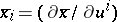
at  . In other words, the spherical map is defined by a multivector constructed from
  independent vectors tangent to
  :
:
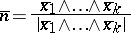 |
(here  are local coordinates of the point
  ,
,  , and
, and  is the position vector of
  ). For example, when
  ,
,
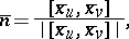 |
where  is the vector product; this simplest case was examined by C.F. Gauss in 1814. The image under the spherical map is called the spherical image of
  .
.
The form
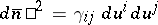 |
is the inverse image of the metric form of  , and is called the third fundamental form of the (hyper)surface
  . Its corresponding tensor
  is related to the tensors
  and
and  of the first and second fundamental forms, respectively, by the relation
 |
while the metric connections corresponding to  and
and  are adjoint connections.
As well as the spherical map, it is useful in the case of a (hyper)surface that is uniquely projected onto a certain (hyper)plane to consider the so-called normal map  . For a (hyper)surface defined by the equation
 |
(here  are Cartesian coordinates in
  ),
),  is defined thus:
 |
where  , so
, so  .
.
For non-orientable (hyper)surfaces, the so-called non-orientable spherical map is used — a mapping from  into the elliptic space
  (which can be interpreted as the set of straight lines that pass through the centre of
  , i.e.
  -dimensional projective space): The line perpendicular to the tangent plane to
  at a point
  is associated with
  .
.
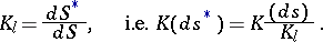
The spherical map characterizes the curvature of a (hyper)surface in a space. Indeed, the ratio of the area elements of the spherical image  and the surface
  itself at the point
  is equal to the total (or Kronecker or outer) curvature
  — the product of the principal curvatures of
  at
at  :
:
 |
In precisely the same way, the (integral) curvature of a set  is equal to the area of its spherical image (i.e. the set
  ):
):
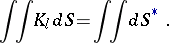 | (1) |
Generalizations of the spherical map.
1) The tangent representation — the spherical map of a submanifold  to
to  — is a mapping
 |
where  is a Grassmann manifold, defined (here) in the following way. Let
  be the tangent space to
  at a point
  , which can be considered as a (hyper)plane in
  , while
  is the
  -dimensional subspace that passes through the origin of
  parallel to
  . The mapping
  is also called the spherical map. A generalization of formula (1) holds for
  even:
even:
 |
here  , where
  is the curvature form on
  ,
,  is the analogous form on
  , and
, and  is the image of
  under the spherical map. The normal map
  has a dual definition: The point
  is associated with the orthogonal complement to
  .
.
2) A Gauss map of a vector bundle  into a vector space
  ,
,  , is an (arbitrary) mapping
 |
from the fibre space  that induces a linear monomorphism on each fibre. For the canonical vector bundle
  (which is the subbundle of the product
  , of which the total space consists of all possible pairs
  with
with  ), the mapping
  is called the canonical Gauss map. For any fibre bundle
  , every Gauss map is a composition of a canonical Gauss map and a morphism of fibre bundles; a Gauss map exists if and only if a mapping
  (where
  is the base of the fibre bundle) exists such that
  and
and  are isomorphic (in particular, for every vector bundle over a paracompact space there is a Gauss map into
  ). For submanifolds of a Riemannian space, there are several generalizations of spherical maps.
3) An Efimov map relates to surfaces  in a Riemannian space
  and is an extension of the above-mentioned concept of adjoint connections. It is defined more formally because of the lack of absolute parallelism in
  and the examination of the analogue of the third fundamental form — the square of the covariant differential of the normal —
  . The relation between the Gaussian curvatures
  and
and  proves to be more complex (a consequence of the inhomogeneity, generally speaking, of the Codazzi equations). This relation remains as before, i.e.
  ; here
  ,
,  are the Gaussian curvatures of the metrics
  and
and  (in the case of
  ,
,  ), and the previous formula
  is obtained, where
  is the exterior curvature of
  in
in  , for example in the following situation: The normal to
  is an eigenvector of the Ricci tensor of the space
  (considered at the points of
  ), in other words,
  is one of the principal surfaces of this tensor. This is always the case if
  is a space of constant curvature.
Finally, the concept of a spherical map is introduced for certain classes of irregular surfaces.
4) The polar mapping is a spherical map from a convex (hyper)surface  into
into  that associates to a point
  the set
  of all unit vectors, drawn from the origin, that are parallel to the normals of the supporting (hyper)planes to
  at
at  . Aleksandrov's theorem: The spherical image
  of every Borel set
  is measurable, and the integral curvature
  is a totally-additive function.
References
| [1] | V.F. Kagan, "Foundations of the theory of surfaces in a tensor setting" , 2 , Moscow-Leningrad (1948) (In Russian) |
| [2] | I.Ya. Bakel'man, A.L. Verner, B.E. Kantor, "Introduction to differential geometry "in the large" " , Moscow (1973) (In Russian) |
| [3] | A.S. Mishchenko, A.T. Fomenko, "A course of differential geometry and topology" , MIR (1988) (Translated from Russian) |
| [4] | A.P. Norden, "Spaces with an affine connection" , Nauka , Moscow-Leningrad (1976) (In Russian) |
| [5] | J.T. Schwartz, "Differential geometry and topology" , Gordon & Breach (1968) |
| [6] | D. Husemoller, "Fibre bundles" , McGraw-Hill (1966) |
| [7] | R.L. Bishop, R.J. Crittenden, "Geometry of manifolds" , Acad. Press (1964) |
| [8] | L.P. Eisenhart, "Riemannian geometry" , Princeton Univ. Press (1949) |
| [9] | H. Busemann, "Convex surfaces" , Interscience (1958) |
Comments
References
| [a1] | M. Spivak, "A comprehensive introduction to differential geometry" , 1979 , Publish or Perish (1975) pp. 1–5 |
Spherical map. Encyclopedia of Mathematics. URL: http://encyclopediaofmath.org/index.php?title=Spherical_map&oldid=18244