Difference between revisions of "Multi-dimensional logarithmic residues"
(Importing text file) |
m (AUTOMATIC EDIT (latexlist): Replaced 57 formulas out of 60 by TEX code with an average confidence of 2.0 and a minimal confidence of 2.0.) |
||
| Line 1: | Line 1: | ||
| + | <!--This article has been texified automatically. Since there was no Nroff source code for this article, | ||
| + | the semi-automatic procedure described at https://encyclopediaofmath.org/wiki/User:Maximilian_Janisch/latexlist | ||
| + | was used. | ||
| + | If the TeX and formula formatting is correct, please remove this message and the {{TEX|semi-auto}} category. | ||
| + | |||
| + | Out of 60 formulas, 57 were replaced by TEX code.--> | ||
| + | |||
| + | {{TEX|semi-auto}}{{TEX|partial}} | ||
By a logarithmic residue formula one usually understands an integral representation for the sum of the values of a holomorphic function at all the zeros of a holomorphic mapping in a given domain, where the number of times each zero is taken is equal to the multiplicity of the zero (for instance, a formula for the number of these zeros). Consider a mapping | By a logarithmic residue formula one usually understands an integral representation for the sum of the values of a holomorphic function at all the zeros of a holomorphic mapping in a given domain, where the number of times each zero is taken is equal to the multiplicity of the zero (for instance, a formula for the number of these zeros). Consider a mapping | ||
| − | + | \begin{equation} \tag{a1} w = f ( z ) \end{equation} | |
| − | which is holomorphic on the closed domain | + | which is holomorphic on the closed domain $\overline{ D }$ and has no zeros on $\partial D$, where $D$ is a bounded domain in $\mathbf{C} ^ { n }$ with piecewise smooth boundary $\partial D$, $w = ( w _ { 1 } , \dots , w _ { n } )$, $z = ( z_ 1 , \dots , z _ { n } )$, $f = ( f _ { 1 } , \dots , f _ { n } )$. Consider a function $\varphi$ holomorphic in $D$ and continuous on $\overline{ D }$. |
| − | The following assertion is due to G. Roos [[#References|[a1]]]: If the vector function | + | The following assertion is due to G. Roos [[#References|[a1]]]: If the vector function $w \in C ^ { ( 1 ) } ( \partial D )$ is such that $\langle w , f \rangle \neq 0$ on $\partial D$, then |
| − | + | \begin{equation} \tag{a2} \frac { ( n - 1 ) ! } { ( 2 \pi i ) ^ {n } } \int _ { \partial D } \varphi \frac { \sum _ { k = 1 } ^ { n } ( - 1 ) ^ { k - 1 } w _ { k } d w [ k ] \wedge d f } { \langle w ,\, f \rangle ^ { n } } = \end{equation} | |
| − | + | \begin{equation*} = \sum _ { a \in Z _ { f } } \varphi ( a ). \end{equation*} | |
| − | Here, | + | Here, $\langle w , f \rangle = w _ { 1 } f _ { 1 } + \ldots + w _ { n } f _ { n }$, $d f = d f _ { 1 } \wedge \ldots \wedge d f _ { n }$, $d w [ k ] = d w _ { 1 } \wedge \ldots \wedge d w _ { k - 1 } \wedge d w _ { k + 1 } \wedge \ldots \wedge d w _ { n }$, and $Z _ { f }$ is the set of zeros of the mapping (a1) in $D$. The sum at the right-hand side of (a2) can be written as integrals of various dimensions from $n$ to $2 n - 1$ [[#References|[a1]]] and in terms of currents, and the corresponding integration is over the whole complex manifold (as in the Poincaré–Lelong formula and for the Coleff–Herrera residue current; [[#References|[a2]]]). |
==Applications.== | ==Applications.== | ||
| Line 18: | Line 26: | ||
Consider the system of algebraic equations | Consider the system of algebraic equations | ||
| − | + | \begin{equation} \tag{a3} f _ { j } = z _ { j } ^ { k _ { j } } + P _ { j } ( z ) , \quad j = 1 , \dots , n, \end{equation} | |
| − | where the degree of | + | where the degree of $p_j$ is less than $ k_{j }$ for $j = 1 , \ldots , n$. |
| − | If | + | If $R ( z )$ is a polynomial of degree $m$, then |
| − | + | \begin{equation} \tag{a4} \sum _ { a \in Z _ { f } } R ( a ) = \end{equation} | |
| − | <table class="eq" style="width:100%;"> <tr><td | + | <table class="eq" style="width:100%;"> <tr><td style="width:94%;text-align:center;" valign="top"><img align="absmiddle" border="0" src="https://www.encyclopediaofmath.org/legacyimages/m/m120/m120270/m12027032.png"/></td> </tr></table> |
| − | where | + | where $\Delta$ is the Jacobian of the system (a3) and $N$ is the linear functional acting on the polynomials in $z _ { 1 } , \dots , z _ { n } , 1 / z _ { 1 } , \dots , 1 / z _ { n }$ by associating to any such polynomial its free term (L. Aizenberg, cf. [[#References|[a1]]]). |
Using formula (a4) one can compute power sums of, for example, the first coordinates of the roots of the system (a3), | Using formula (a4) one can compute power sums of, for example, the first coordinates of the roots of the system (a3), | ||
| − | + | \begin{equation*} s _ { j } = \sum _ { \text{l} = 1 } ^ { M } ( z _ { 1 } ^ { ( \text{l} ) } ) ^ { j } , \quad j = 1 , \ldots , M, \end{equation*} | |
| − | where | + | where $M$ is the number of roots. The coefficients of the polynomial $\Gamma ( z _ { 1 } ) = z _ { 1 } ^ { M } + b _ { 1 } z _ { 1 } ^ { M - 1 } + \ldots + b _ { M - 1 } z _ { 1 } + b _ { M }$, having roots $z _ { 1 } ^ { ( 1 ) } , \dots , z _ { 1 } ^ { ( M ) }$, are given by Waring's formula or Newton's recurrence formula. Thus, one has obtained a new method for eliminating unknowns; this method does not add extra roots and does not omit any root. This method appears to be simpler than the classical methods of elimination using the resultants of polynomials. Formula (a4) leads to a particularly simple computation when the degree of the polynomial $R ( z )$ is small. |
===Example.=== | ===Example.=== | ||
| − | Consider in | + | Consider in $\mathbf{R} ^ { 3 }$ the three surfaces of third order |
| − | + | \begin{equation} \tag{a5} \left\{ \begin{array} { l } { x _ { 1 } ^ { 3 } + \sum _ { i + j + k \leq 2 } a _ { i j k } x _ { 1 } ^ { i } x _ { 2 } ^ { j } x _ { 3 } ^ { k } = 0, } \\ { x _ { 2 } ^ { 3 } + \sum _ { i + j + k \leq 2 } b _ { i j k } x _ { 1 } ^ { i } x _ { 2 } ^ { j } x _ { 3 } ^ { k } = 0, } \\ { x _ { 3 } ^ { 3 } + \sum _ { i + j + k \leq 2 } c _ { i j k } x _ { 1 } ^ { i } x _ { 2 } ^ { j } x _ { 3 } ^ { k } = 0, } \end{array} \right. \end{equation} | |
| − | where | + | where $a _ {i j k }$, $b _ { i j k }$ and $c_{i j k}$ are real numbers. Let the surfaces in (a5) be in "general position" in the sense that they have $27$ points in common in $\mathbf{R} ^ { 3 }$, the maximum possible number. Fix a point $( A , B , C ) \in \textbf{R} ^ { 3 }$ and compute, using (a4), the sum of the squares of the distances from this point to the $27$ common points of the surfaces (a5). This sum is equal to <img align="absmiddle" border="0" src="https://www.encyclopediaofmath.org/legacyimages/m/m120/m120270/m12027050.png"/>. If is curious that the answer does not depend on $12$ of the $30$ coefficients of the equations of the surfaces (a5). |
==Generalization.== | ==Generalization.== | ||
There exists a more general formula than (a4) for systems of algebraic equations | There exists a more general formula than (a4) for systems of algebraic equations | ||
| − | + | \begin{equation} \tag{a6} Q _ { j } ( z ) + P _ { j } ( z ) = 0 , \quad j = 1 , \dots , n, \end{equation} | |
| − | where the | + | where the $Q _ { j } ( z )$ are homogeneous polynomials with $ k_{j }$ as their highest degree while the degree of each $P_{j}$ is less than $ k_{j }$, $j = 1 , \ldots , n$. It is assumed that the only common zero of the polynomials $Q_{j}$ is the origin (see [[#References|[a1]]]). This generalized formula for system (a6) has found application in the determination of all stationary solutions of certain chemical kinetic equations [[#References|[a3]]]. |
====References==== | ====References==== | ||
| − | <table>< | + | <table><tr><td valign="top">[a1]</td> <td valign="top"> L. Aizenberg, A.P. Yuzhakov, "Integral representation and residues in multidimensional complex analysis" , Amer. Math. Soc. (1983)</td></tr><tr><td valign="top">[a2]</td> <td valign="top"> L. Aizenberg, A.P. Yuzhakov, A.K. Tsikh, "Multidimensional residues and applications" , ''Several complex variables, II'' , ''Encycl. Math. Sci.'' , '''8''' , Springer (1994) pp. 1–58</td></tr><tr><td valign="top">[a3]</td> <td valign="top"> V.I. Bykov, A.M. Kytmanov, M.Z. Lazman, "Elimination method in computer algebra of polynomials" , Kluwer Acad. Publ. (1997)</td></tr></table> |
Revision as of 15:30, 1 July 2020
By a logarithmic residue formula one usually understands an integral representation for the sum of the values of a holomorphic function at all the zeros of a holomorphic mapping in a given domain, where the number of times each zero is taken is equal to the multiplicity of the zero (for instance, a formula for the number of these zeros). Consider a mapping
\begin{equation} \tag{a1} w = f ( z ) \end{equation}
which is holomorphic on the closed domain $\overline{ D }$ and has no zeros on $\partial D$, where $D$ is a bounded domain in $\mathbf{C} ^ { n }$ with piecewise smooth boundary $\partial D$, $w = ( w _ { 1 } , \dots , w _ { n } )$, $z = ( z_ 1 , \dots , z _ { n } )$, $f = ( f _ { 1 } , \dots , f _ { n } )$. Consider a function $\varphi$ holomorphic in $D$ and continuous on $\overline{ D }$.
The following assertion is due to G. Roos [a1]: If the vector function $w \in C ^ { ( 1 ) } ( \partial D )$ is such that $\langle w , f \rangle \neq 0$ on $\partial D$, then
\begin{equation} \tag{a2} \frac { ( n - 1 ) ! } { ( 2 \pi i ) ^ {n } } \int _ { \partial D } \varphi \frac { \sum _ { k = 1 } ^ { n } ( - 1 ) ^ { k - 1 } w _ { k } d w [ k ] \wedge d f } { \langle w ,\, f \rangle ^ { n } } = \end{equation}
\begin{equation*} = \sum _ { a \in Z _ { f } } \varphi ( a ). \end{equation*}
Here, $\langle w , f \rangle = w _ { 1 } f _ { 1 } + \ldots + w _ { n } f _ { n }$, $d f = d f _ { 1 } \wedge \ldots \wedge d f _ { n }$, $d w [ k ] = d w _ { 1 } \wedge \ldots \wedge d w _ { k - 1 } \wedge d w _ { k + 1 } \wedge \ldots \wedge d w _ { n }$, and $Z _ { f }$ is the set of zeros of the mapping (a1) in $D$. The sum at the right-hand side of (a2) can be written as integrals of various dimensions from $n$ to $2 n - 1$ [a1] and in terms of currents, and the corresponding integration is over the whole complex manifold (as in the Poincaré–Lelong formula and for the Coleff–Herrera residue current; [a2]).
Applications.
Applications of multi-dimensional logarithmic residues to series expansion of implicit functions, the computation of the zero-multiplicity of a holomorphic mapping and to the theory of numbers are given in [a1], [a2].
Consider the system of algebraic equations
\begin{equation} \tag{a3} f _ { j } = z _ { j } ^ { k _ { j } } + P _ { j } ( z ) , \quad j = 1 , \dots , n, \end{equation}
where the degree of $p_j$ is less than $ k_{j }$ for $j = 1 , \ldots , n$.
If $R ( z )$ is a polynomial of degree $m$, then
\begin{equation} \tag{a4} \sum _ { a \in Z _ { f } } R ( a ) = \end{equation}
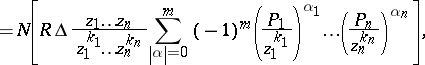 |
where $\Delta$ is the Jacobian of the system (a3) and $N$ is the linear functional acting on the polynomials in $z _ { 1 } , \dots , z _ { n } , 1 / z _ { 1 } , \dots , 1 / z _ { n }$ by associating to any such polynomial its free term (L. Aizenberg, cf. [a1]).
Using formula (a4) one can compute power sums of, for example, the first coordinates of the roots of the system (a3),
\begin{equation*} s _ { j } = \sum _ { \text{l} = 1 } ^ { M } ( z _ { 1 } ^ { ( \text{l} ) } ) ^ { j } , \quad j = 1 , \ldots , M, \end{equation*}
where $M$ is the number of roots. The coefficients of the polynomial $\Gamma ( z _ { 1 } ) = z _ { 1 } ^ { M } + b _ { 1 } z _ { 1 } ^ { M - 1 } + \ldots + b _ { M - 1 } z _ { 1 } + b _ { M }$, having roots $z _ { 1 } ^ { ( 1 ) } , \dots , z _ { 1 } ^ { ( M ) }$, are given by Waring's formula or Newton's recurrence formula. Thus, one has obtained a new method for eliminating unknowns; this method does not add extra roots and does not omit any root. This method appears to be simpler than the classical methods of elimination using the resultants of polynomials. Formula (a4) leads to a particularly simple computation when the degree of the polynomial $R ( z )$ is small.
Example.
Consider in $\mathbf{R} ^ { 3 }$ the three surfaces of third order
\begin{equation} \tag{a5} \left\{ \begin{array} { l } { x _ { 1 } ^ { 3 } + \sum _ { i + j + k \leq 2 } a _ { i j k } x _ { 1 } ^ { i } x _ { 2 } ^ { j } x _ { 3 } ^ { k } = 0, } \\ { x _ { 2 } ^ { 3 } + \sum _ { i + j + k \leq 2 } b _ { i j k } x _ { 1 } ^ { i } x _ { 2 } ^ { j } x _ { 3 } ^ { k } = 0, } \\ { x _ { 3 } ^ { 3 } + \sum _ { i + j + k \leq 2 } c _ { i j k } x _ { 1 } ^ { i } x _ { 2 } ^ { j } x _ { 3 } ^ { k } = 0, } \end{array} \right. \end{equation}
where $a _ {i j k }$, $b _ { i j k }$ and $c_{i j k}$ are real numbers. Let the surfaces in (a5) be in "general position" in the sense that they have $27$ points in common in $\mathbf{R} ^ { 3 }$, the maximum possible number. Fix a point $( A , B , C ) \in \textbf{R} ^ { 3 }$ and compute, using (a4), the sum of the squares of the distances from this point to the $27$ common points of the surfaces (a5). This sum is equal to  . If is curious that the answer does not depend on $12$ of the $30$ coefficients of the equations of the surfaces (a5).
Generalization.
There exists a more general formula than (a4) for systems of algebraic equations
\begin{equation} \tag{a6} Q _ { j } ( z ) + P _ { j } ( z ) = 0 , \quad j = 1 , \dots , n, \end{equation}
where the $Q _ { j } ( z )$ are homogeneous polynomials with $ k_{j }$ as their highest degree while the degree of each $P_{j}$ is less than $ k_{j }$, $j = 1 , \ldots , n$. It is assumed that the only common zero of the polynomials $Q_{j}$ is the origin (see [a1]). This generalized formula for system (a6) has found application in the determination of all stationary solutions of certain chemical kinetic equations [a3].
References
| [a1] | L. Aizenberg, A.P. Yuzhakov, "Integral representation and residues in multidimensional complex analysis" , Amer. Math. Soc. (1983) |
| [a2] | L. Aizenberg, A.P. Yuzhakov, A.K. Tsikh, "Multidimensional residues and applications" , Several complex variables, II , Encycl. Math. Sci. , 8 , Springer (1994) pp. 1–58 |
| [a3] | V.I. Bykov, A.M. Kytmanov, M.Z. Lazman, "Elimination method in computer algebra of polynomials" , Kluwer Acad. Publ. (1997) |
Multi-dimensional logarithmic residues. Encyclopedia of Mathematics. URL: http://encyclopediaofmath.org/index.php?title=Multi-dimensional_logarithmic_residues&oldid=14334