Difference between revisions of "Markov process"
Ulf Rehmann (talk | contribs) m (Undo revision 37893 by Ulf Rehmann (talk)) |
Ulf Rehmann (talk | contribs) m (Reverted edits by Ulf Rehmann (talk) to last revision by Boris Tsirelson) |
||
| Line 1: | Line 1: | ||
| − | + | ''process without after-effects'' | |
| + | |||
| + | {{MSC|60Jxx}} | ||
| + | |||
| + | [[Category:Markov processes]] | ||
| + | |||
| + | A [[Stochastic process|stochastic process]] whose evolution after a given time <img align="absmiddle" border="0" src="https://www.encyclopediaofmath.org/legacyimages/m/m062/m062490/m0624901.png" /> does not depend on the evolution before <img align="absmiddle" border="0" src="https://www.encyclopediaofmath.org/legacyimages/m/m062/m062490/m0624902.png" />, given that the value of the process at <img align="absmiddle" border="0" src="https://www.encyclopediaofmath.org/legacyimages/m/m062/m062490/m0624903.png" /> is fixed (briefly; the "future" and "past" of the process are independent of each other for a known "present" ). | ||
| + | |||
| + | The defining property of a Markov process is commonly called the [[Markov property|Markov property]]; it was first stated by A.A. Markov . However, in the work of L. Bachelier it is already possible to find an attempt to discuss [[Brownian motion|Brownian motion]] as a Markov process, an attempt which received justification later in the research of N. Wiener (1923). The basis of the general theory of continuous-time Markov processes was laid by A.N. Kolmogorov . | ||
| + | |||
| + | ==The Markov property.== | ||
| + | There are essentially distinct definitions of a Markov process. One of the more widely used is the following. On a [[Probability space|probability space]] <img align="absmiddle" border="0" src="https://www.encyclopediaofmath.org/legacyimages/m/m062/m062490/m0624904.png" /> let there be given a stochastic process <img align="absmiddle" border="0" src="https://www.encyclopediaofmath.org/legacyimages/m/m062/m062490/m0624905.png" />, <img align="absmiddle" border="0" src="https://www.encyclopediaofmath.org/legacyimages/m/m062/m062490/m0624906.png" />, taking values in a [[Measurable space|measurable space]] <img align="absmiddle" border="0" src="https://www.encyclopediaofmath.org/legacyimages/m/m062/m062490/m0624907.png" />, where <img align="absmiddle" border="0" src="https://www.encyclopediaofmath.org/legacyimages/m/m062/m062490/m0624908.png" /> is a subset of the real line <img align="absmiddle" border="0" src="https://www.encyclopediaofmath.org/legacyimages/m/m062/m062490/m0624909.png" />. Let <img align="absmiddle" border="0" src="https://www.encyclopediaofmath.org/legacyimages/m/m062/m062490/m06249010.png" /> (respectively, <img align="absmiddle" border="0" src="https://www.encyclopediaofmath.org/legacyimages/m/m062/m062490/m06249011.png" />) be the <img align="absmiddle" border="0" src="https://www.encyclopediaofmath.org/legacyimages/m/m062/m062490/m06249012.png" />-algebra in <img align="absmiddle" border="0" src="https://www.encyclopediaofmath.org/legacyimages/m/m062/m062490/m06249013.png" /> generated by the variables <img align="absmiddle" border="0" src="https://www.encyclopediaofmath.org/legacyimages/m/m062/m062490/m06249014.png" /> for <img align="absmiddle" border="0" src="https://www.encyclopediaofmath.org/legacyimages/m/m062/m062490/m06249015.png" /> (<img align="absmiddle" border="0" src="https://www.encyclopediaofmath.org/legacyimages/m/m062/m062490/m06249016.png" />), where <img align="absmiddle" border="0" src="https://www.encyclopediaofmath.org/legacyimages/m/m062/m062490/m06249017.png" />. In other words, <img align="absmiddle" border="0" src="https://www.encyclopediaofmath.org/legacyimages/m/m062/m062490/m06249018.png" /> (respectively, <img align="absmiddle" border="0" src="https://www.encyclopediaofmath.org/legacyimages/m/m062/m062490/m06249019.png" />) is the collection of events connected with the evolution of the process up to time (starting from time) <img align="absmiddle" border="0" src="https://www.encyclopediaofmath.org/legacyimages/m/m062/m062490/m06249020.png" />. <img align="absmiddle" border="0" src="https://www.encyclopediaofmath.org/legacyimages/m/m062/m062490/m06249021.png" /> is called a Markov process if (almost certainly) for all <img align="absmiddle" border="0" src="https://www.encyclopediaofmath.org/legacyimages/m/m062/m062490/m06249022.png" />, <img align="absmiddle" border="0" src="https://www.encyclopediaofmath.org/legacyimages/m/m062/m062490/m06249023.png" /> the Markov property | ||
| + | |||
| + | <table class="eq" style="width:100%;"> <tr><td valign="top" style="width:94%;text-align:center;"><img align="absmiddle" border="0" src="https://www.encyclopediaofmath.org/legacyimages/m/m062/m062490/m06249024.png" /></td> <td valign="top" style="width:5%;text-align:right;">(1)</td></tr></table> | ||
| + | |||
| + | holds, or, what is the same, if for any <img align="absmiddle" border="0" src="https://www.encyclopediaofmath.org/legacyimages/m/m062/m062490/m06249025.png" /> and <img align="absmiddle" border="0" src="https://www.encyclopediaofmath.org/legacyimages/m/m062/m062490/m06249026.png" />, | ||
| + | |||
| + | <table class="eq" style="width:100%;"> <tr><td valign="top" style="width:94%;text-align:center;"><img align="absmiddle" border="0" src="https://www.encyclopediaofmath.org/legacyimages/m/m062/m062490/m06249027.png" /></td> <td valign="top" style="width:5%;text-align:right;">(2)</td></tr></table> | ||
| + | |||
| + | A Markov process for which <img align="absmiddle" border="0" src="https://www.encyclopediaofmath.org/legacyimages/m/m062/m062490/m06249028.png" /> is contained in the natural numbers is called a [[Markov chain|Markov chain]] (however, the latter term is mostly associated with the case of an at most countable <img align="absmiddle" border="0" src="https://www.encyclopediaofmath.org/legacyimages/m/m062/m062490/m06249029.png" />). If <img align="absmiddle" border="0" src="https://www.encyclopediaofmath.org/legacyimages/m/m062/m062490/m06249030.png" /> is an interval in <img align="absmiddle" border="0" src="https://www.encyclopediaofmath.org/legacyimages/m/m062/m062490/m06249031.png" /> and <img align="absmiddle" border="0" src="https://www.encyclopediaofmath.org/legacyimages/m/m062/m062490/m06249032.png" /> is at most countable, a Markov process is called a continuous-time Markov chain. Examples of continuous-time Markov processes are furnished by diffusion processes (cf. [[Diffusion process|Diffusion process]]) and processes with independent increments (cf. [[Stochastic process with independent increments|Stochastic process with independent increments]]), including Poisson and Wiener processes (cf. [[Poisson process|Poisson process]]; [[Wiener process|Wiener process]]). | ||
| + | |||
| + | In what follows the discussion will concern only the case <img align="absmiddle" border="0" src="https://www.encyclopediaofmath.org/legacyimages/m/m062/m062490/m06249033.png" />, for the sake of being specific. The formulas (1) and (2) give an explicit interpretation of the principle of independence of "past" and "future" events when the "present" is known, but the definition of Markov process based on them has proved to be insufficiently flexible in the numerous situations where one is obliged to consider not one, but a collection of conditions of the type (1) or (2) corresponding to different, but in some sense consistent, measures <img align="absmiddle" border="0" src="https://www.encyclopediaofmath.org/legacyimages/m/m062/m062490/m06249034.png" />. Such reasoning has led to the acceptance of the following definitions (see , ). | ||
| + | |||
| + | Suppose one is given: | ||
| + | |||
| + | a) a measurable space <img align="absmiddle" border="0" src="https://www.encyclopediaofmath.org/legacyimages/m/m062/m062490/m06249035.png" />, where the <img align="absmiddle" border="0" src="https://www.encyclopediaofmath.org/legacyimages/m/m062/m062490/m06249036.png" />-algebra <img align="absmiddle" border="0" src="https://www.encyclopediaofmath.org/legacyimages/m/m062/m062490/m06249037.png" /> contains all one-point sets in <img align="absmiddle" border="0" src="https://www.encyclopediaofmath.org/legacyimages/m/m062/m062490/m06249038.png" />; | ||
| + | |||
| + | b) a measurable space <img align="absmiddle" border="0" src="https://www.encyclopediaofmath.org/legacyimages/m/m062/m062490/m06249039.png" />, equipped with a family of <img align="absmiddle" border="0" src="https://www.encyclopediaofmath.org/legacyimages/m/m062/m062490/m06249040.png" />-algebras <img align="absmiddle" border="0" src="https://www.encyclopediaofmath.org/legacyimages/m/m062/m062490/m06249041.png" />, <img align="absmiddle" border="0" src="https://www.encyclopediaofmath.org/legacyimages/m/m062/m062490/m06249042.png" />, such that <img align="absmiddle" border="0" src="https://www.encyclopediaofmath.org/legacyimages/m/m062/m062490/m06249043.png" /> if <img align="absmiddle" border="0" src="https://www.encyclopediaofmath.org/legacyimages/m/m062/m062490/m06249044.png" />; | ||
| + | |||
| + | c) a function ( "trajectory" ) <img align="absmiddle" border="0" src="https://www.encyclopediaofmath.org/legacyimages/m/m062/m062490/m06249045.png" />, defining for <img align="absmiddle" border="0" src="https://www.encyclopediaofmath.org/legacyimages/m/m062/m062490/m06249046.png" /> and <img align="absmiddle" border="0" src="https://www.encyclopediaofmath.org/legacyimages/m/m062/m062490/m06249047.png" /> a [[Measurable mapping|measurable mapping]] from <img align="absmiddle" border="0" src="https://www.encyclopediaofmath.org/legacyimages/m/m062/m062490/m06249048.png" /> to <img align="absmiddle" border="0" src="https://www.encyclopediaofmath.org/legacyimages/m/m062/m062490/m06249049.png" />; | ||
| + | |||
| + | d) for each <img align="absmiddle" border="0" src="https://www.encyclopediaofmath.org/legacyimages/m/m062/m062490/m06249050.png" /> and <img align="absmiddle" border="0" src="https://www.encyclopediaofmath.org/legacyimages/m/m062/m062490/m06249051.png" /> a [[Probability measure|probability measure]] <img align="absmiddle" border="0" src="https://www.encyclopediaofmath.org/legacyimages/m/m062/m062490/m06249052.png" /> on the <img align="absmiddle" border="0" src="https://www.encyclopediaofmath.org/legacyimages/m/m062/m062490/m06249053.png" />-algebra <img align="absmiddle" border="0" src="https://www.encyclopediaofmath.org/legacyimages/m/m062/m062490/m06249054.png" /> such that the function <img align="absmiddle" border="0" src="https://www.encyclopediaofmath.org/legacyimages/m/m062/m062490/m06249055.png" /> is measurable with respect to <img align="absmiddle" border="0" src="https://www.encyclopediaofmath.org/legacyimages/m/m062/m062490/m06249056.png" />, if <img align="absmiddle" border="0" src="https://www.encyclopediaofmath.org/legacyimages/m/m062/m062490/m06249057.png" /> and <img align="absmiddle" border="0" src="https://www.encyclopediaofmath.org/legacyimages/m/m062/m062490/m06249058.png" />. | ||
| + | |||
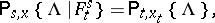
| + | The collection <img align="absmiddle" border="0" src="https://www.encyclopediaofmath.org/legacyimages/m/m062/m062490/m06249059.png" /> is called a (non-terminating) Markov process given on <img align="absmiddle" border="0" src="https://www.encyclopediaofmath.org/legacyimages/m/m062/m062490/m06249060.png" /> if <img align="absmiddle" border="0" src="https://www.encyclopediaofmath.org/legacyimages/m/m062/m062490/m06249061.png" />-almost certainly | ||
| + | |||
| + | <table class="eq" style="width:100%;"> <tr><td valign="top" style="width:94%;text-align:center;"><img align="absmiddle" border="0" src="https://www.encyclopediaofmath.org/legacyimages/m/m062/m062490/m06249062.png" /></td> <td valign="top" style="width:5%;text-align:right;">(3)</td></tr></table> | ||
| + | |||
| + | for any <img align="absmiddle" border="0" src="https://www.encyclopediaofmath.org/legacyimages/m/m062/m062490/m06249063.png" /> and <img align="absmiddle" border="0" src="https://www.encyclopediaofmath.org/legacyimages/m/m062/m062490/m06249064.png" />. Here <img align="absmiddle" border="0" src="https://www.encyclopediaofmath.org/legacyimages/m/m062/m062490/m06249065.png" /> is the space of elementary events, <img align="absmiddle" border="0" src="https://www.encyclopediaofmath.org/legacyimages/m/m062/m062490/m06249066.png" /> is the phase space or state space and <img align="absmiddle" border="0" src="https://www.encyclopediaofmath.org/legacyimages/m/m062/m062490/m06249067.png" /> is the [[Transition function|transition function]] or transition probability of <img align="absmiddle" border="0" src="https://www.encyclopediaofmath.org/legacyimages/m/m062/m062490/m06249068.png" />. If <img align="absmiddle" border="0" src="https://www.encyclopediaofmath.org/legacyimages/m/m062/m062490/m06249069.png" /> is endowed with a topology and <img align="absmiddle" border="0" src="https://www.encyclopediaofmath.org/legacyimages/m/m062/m062490/m06249070.png" /> is the collection of Borel sets in <img align="absmiddle" border="0" src="https://www.encyclopediaofmath.org/legacyimages/m/m062/m062490/m06249071.png" />, then it is commonly said that the Markov process is given on <img align="absmiddle" border="0" src="https://www.encyclopediaofmath.org/legacyimages/m/m062/m062490/m06249072.png" />. Usually included in the definition of a Markov process is the requirement that <img align="absmiddle" border="0" src="https://www.encyclopediaofmath.org/legacyimages/m/m062/m062490/m06249073.png" />, and then <img align="absmiddle" border="0" src="https://www.encyclopediaofmath.org/legacyimages/m/m062/m062490/m06249074.png" />, <img align="absmiddle" border="0" src="https://www.encyclopediaofmath.org/legacyimages/m/m062/m062490/m06249075.png" />, is interpreted as the probability of <img align="absmiddle" border="0" src="https://www.encyclopediaofmath.org/legacyimages/m/m062/m062490/m06249076.png" /> under the condition that <img align="absmiddle" border="0" src="https://www.encyclopediaofmath.org/legacyimages/m/m062/m062490/m06249077.png" />. | ||
| + | |||
| + | The following question arises: Is every Markov transition function <img align="absmiddle" border="0" src="https://www.encyclopediaofmath.org/legacyimages/m/m062/m062490/m06249078.png" />, given on a measurable space <img align="absmiddle" border="0" src="https://www.encyclopediaofmath.org/legacyimages/m/m062/m062490/m06249079.png" />, the transition function of some Markov process? The answer is affirmative if, for example, <img align="absmiddle" border="0" src="https://www.encyclopediaofmath.org/legacyimages/m/m062/m062490/m06249080.png" /> is a separable, locally compact space and <img align="absmiddle" border="0" src="https://www.encyclopediaofmath.org/legacyimages/m/m062/m062490/m06249081.png" /> is the family of Borel sets in <img align="absmiddle" border="0" src="https://www.encyclopediaofmath.org/legacyimages/m/m062/m062490/m06249082.png" />. In addition, let <img align="absmiddle" border="0" src="https://www.encyclopediaofmath.org/legacyimages/m/m062/m062490/m06249083.png" /> be a complete metric space and let | ||
| + | |||
| + | <table class="eq" style="width:100%;"> <tr><td valign="top" style="width:94%;text-align:center;"><img align="absmiddle" border="0" src="https://www.encyclopediaofmath.org/legacyimages/m/m062/m062490/m06249084.png" /></td> </tr></table> | ||
| + | |||
| + | for any <img align="absmiddle" border="0" src="https://www.encyclopediaofmath.org/legacyimages/m/m062/m062490/m06249085.png" />, where | ||
| + | |||
| + | <table class="eq" style="width:100%;"> <tr><td valign="top" style="width:94%;text-align:center;"><img align="absmiddle" border="0" src="https://www.encyclopediaofmath.org/legacyimages/m/m062/m062490/m06249086.png" /></td> </tr></table> | ||
| + | |||
| + | and <img align="absmiddle" border="0" src="https://www.encyclopediaofmath.org/legacyimages/m/m062/m062490/m06249087.png" /> is the complement of the <img align="absmiddle" border="0" src="https://www.encyclopediaofmath.org/legacyimages/m/m062/m062490/m06249088.png" />-neighbourhood of <img align="absmiddle" border="0" src="https://www.encyclopediaofmath.org/legacyimages/m/m062/m062490/m06249089.png" />. Then the corresponding Markov process can be taken to be right-continuous and having left limits (that is, its trajectories can be chosen so). The existence of a continuous Markov process is guaranteed by the condition <img align="absmiddle" border="0" src="https://www.encyclopediaofmath.org/legacyimages/m/m062/m062490/m06249090.png" /> as <img align="absmiddle" border="0" src="https://www.encyclopediaofmath.org/legacyimages/m/m062/m062490/m06249091.png" /> (see , ). | ||
| + | |||
| + | In the theory of Markov processes most attention is given to homogeneous (in time) processes. The corresponding definition assumes one is given a system of objects a)–d) with the difference that the parameters <img align="absmiddle" border="0" src="https://www.encyclopediaofmath.org/legacyimages/m/m062/m062490/m06249092.png" /> and <img align="absmiddle" border="0" src="https://www.encyclopediaofmath.org/legacyimages/m/m062/m062490/m06249093.png" /> may now only take the value 0. Even the notation can be simplified: | ||
| + | |||
| + | <table class="eq" style="width:100%;"> <tr><td valign="top" style="width:94%;text-align:center;"><img align="absmiddle" border="0" src="https://www.encyclopediaofmath.org/legacyimages/m/m062/m062490/m06249094.png" /></td> </tr></table> | ||
| + | |||
| + | <table class="eq" style="width:100%;"> <tr><td valign="top" style="width:94%;text-align:center;"><img align="absmiddle" border="0" src="https://www.encyclopediaofmath.org/legacyimages/m/m062/m062490/m06249095.png" /></td> </tr></table> | ||
| + | |||
| + | Subsequently, homogeneity of <img align="absmiddle" border="0" src="https://www.encyclopediaofmath.org/legacyimages/m/m062/m062490/m06249096.png" /> is assumed. That is, it is required that for any <img align="absmiddle" border="0" src="https://www.encyclopediaofmath.org/legacyimages/m/m062/m062490/m06249097.png" /> and <img align="absmiddle" border="0" src="https://www.encyclopediaofmath.org/legacyimages/m/m062/m062490/m06249098.png" /> there is an <img align="absmiddle" border="0" src="https://www.encyclopediaofmath.org/legacyimages/m/m062/m062490/m06249099.png" /> such that <img align="absmiddle" border="0" src="https://www.encyclopediaofmath.org/legacyimages/m/m062/m062490/m062490100.png" /> for <img align="absmiddle" border="0" src="https://www.encyclopediaofmath.org/legacyimages/m/m062/m062490/m062490101.png" />. Because of this, on the <img align="absmiddle" border="0" src="https://www.encyclopediaofmath.org/legacyimages/m/m062/m062490/m062490102.png" />-algebra <img align="absmiddle" border="0" src="https://www.encyclopediaofmath.org/legacyimages/m/m062/m062490/m062490103.png" />, the smallest <img align="absmiddle" border="0" src="https://www.encyclopediaofmath.org/legacyimages/m/m062/m062490/m062490104.png" />-algebra in <img align="absmiddle" border="0" src="https://www.encyclopediaofmath.org/legacyimages/m/m062/m062490/m062490105.png" /> containing the events <img align="absmiddle" border="0" src="https://www.encyclopediaofmath.org/legacyimages/m/m062/m062490/m062490106.png" />, the time shift operators <img align="absmiddle" border="0" src="https://www.encyclopediaofmath.org/legacyimages/m/m062/m062490/m062490107.png" /> are defined, which preserve the operations of union, intersection and difference of sets, and for which | ||
| + | |||
| + | <table class="eq" style="width:100%;"> <tr><td valign="top" style="width:94%;text-align:center;"><img align="absmiddle" border="0" src="https://www.encyclopediaofmath.org/legacyimages/m/m062/m062490/m062490108.png" /></td> </tr></table> | ||
| + | |||
| + | where <img align="absmiddle" border="0" src="https://www.encyclopediaofmath.org/legacyimages/m/m062/m062490/m062490109.png" />, <img align="absmiddle" border="0" src="https://www.encyclopediaofmath.org/legacyimages/m/m062/m062490/m062490110.png" />. | ||
| + | |||
| + | The collection <img align="absmiddle" border="0" src="https://www.encyclopediaofmath.org/legacyimages/m/m062/m062490/m062490111.png" /> is called a (non-terminating) homogeneous Markov process given on <img align="absmiddle" border="0" src="https://www.encyclopediaofmath.org/legacyimages/m/m062/m062490/m062490112.png" /> if <img align="absmiddle" border="0" src="https://www.encyclopediaofmath.org/legacyimages/m/m062/m062490/m062490113.png" />-almost certainly | ||
| + | |||
| + | <table class="eq" style="width:100%;"> <tr><td valign="top" style="width:94%;text-align:center;"><img align="absmiddle" border="0" src="https://www.encyclopediaofmath.org/legacyimages/m/m062/m062490/m062490114.png" /></td> <td valign="top" style="width:5%;text-align:right;">(4)</td></tr></table> | ||
| + | |||
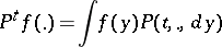
| + | for <img align="absmiddle" border="0" src="https://www.encyclopediaofmath.org/legacyimages/m/m062/m062490/m062490115.png" />, <img align="absmiddle" border="0" src="https://www.encyclopediaofmath.org/legacyimages/m/m062/m062490/m062490116.png" /> and <img align="absmiddle" border="0" src="https://www.encyclopediaofmath.org/legacyimages/m/m062/m062490/m062490117.png" />. The transition function of <img align="absmiddle" border="0" src="https://www.encyclopediaofmath.org/legacyimages/m/m062/m062490/m062490118.png" /> is taken to be <img align="absmiddle" border="0" src="https://www.encyclopediaofmath.org/legacyimages/m/m062/m062490/m062490119.png" />, where, unless otherwise indicated, it is required that <img align="absmiddle" border="0" src="https://www.encyclopediaofmath.org/legacyimages/m/m062/m062490/m062490120.png" />. It is useful to bear in mind that in the verification of (4) it is only necessary to consider sets of the form <img align="absmiddle" border="0" src="https://www.encyclopediaofmath.org/legacyimages/m/m062/m062490/m062490121.png" />, where <img align="absmiddle" border="0" src="https://www.encyclopediaofmath.org/legacyimages/m/m062/m062490/m062490122.png" />, <img align="absmiddle" border="0" src="https://www.encyclopediaofmath.org/legacyimages/m/m062/m062490/m062490123.png" />, and in (4), <img align="absmiddle" border="0" src="https://www.encyclopediaofmath.org/legacyimages/m/m062/m062490/m062490124.png" /> may always replaced by the <img align="absmiddle" border="0" src="https://www.encyclopediaofmath.org/legacyimages/m/m062/m062490/m062490125.png" />-algebra <img align="absmiddle" border="0" src="https://www.encyclopediaofmath.org/legacyimages/m/m062/m062490/m062490126.png" /> equal to the intersection of the completions of <img align="absmiddle" border="0" src="https://www.encyclopediaofmath.org/legacyimages/m/m062/m062490/m062490127.png" /> relative to all possible measures <img align="absmiddle" border="0" src="https://www.encyclopediaofmath.org/legacyimages/m/m062/m062490/m062490128.png" />. Often, one fixes on <img align="absmiddle" border="0" src="https://www.encyclopediaofmath.org/legacyimages/m/m062/m062490/m062490129.png" /> a probability measure <img align="absmiddle" border="0" src="https://www.encyclopediaofmath.org/legacyimages/m/m062/m062490/m062490130.png" /> (the "initial distribution" ) and considers a random Markov function <img align="absmiddle" border="0" src="https://www.encyclopediaofmath.org/legacyimages/m/m062/m062490/m062490131.png" />, where <img align="absmiddle" border="0" src="https://www.encyclopediaofmath.org/legacyimages/m/m062/m062490/m062490132.png" /> is the measure on <img align="absmiddle" border="0" src="https://www.encyclopediaofmath.org/legacyimages/m/m062/m062490/m062490133.png" /> given by | ||
| + | |||
| + | <table class="eq" style="width:100%;"> <tr><td valign="top" style="width:94%;text-align:center;"><img align="absmiddle" border="0" src="https://www.encyclopediaofmath.org/legacyimages/m/m062/m062490/m062490134.png" /></td> </tr></table> | ||
| + | |||
| + | A Markov process <img align="absmiddle" border="0" src="https://www.encyclopediaofmath.org/legacyimages/m/m062/m062490/m062490135.png" /> is called progressively measurable if for each <img align="absmiddle" border="0" src="https://www.encyclopediaofmath.org/legacyimages/m/m062/m062490/m062490136.png" /> the function <img align="absmiddle" border="0" src="https://www.encyclopediaofmath.org/legacyimages/m/m062/m062490/m062490137.png" /> induces a measurable mapping from <img align="absmiddle" border="0" src="https://www.encyclopediaofmath.org/legacyimages/m/m062/m062490/m062490138.png" /> to <img align="absmiddle" border="0" src="https://www.encyclopediaofmath.org/legacyimages/m/m062/m062490/m062490139.png" />, where <img align="absmiddle" border="0" src="https://www.encyclopediaofmath.org/legacyimages/m/m062/m062490/m062490140.png" /> is the <img align="absmiddle" border="0" src="https://www.encyclopediaofmath.org/legacyimages/m/m062/m062490/m062490141.png" />-algebra of Borel subsets of <img align="absmiddle" border="0" src="https://www.encyclopediaofmath.org/legacyimages/m/m062/m062490/m062490142.png" />. A right-continuous Markov process is progressively measurable. There is a method for reducing the non-homogeneous case to the homogeneous case (see ), and in what follows homogeneous Markov processes will be discussed. | ||
| + | |||
| + | ==The strong Markov property.== | ||
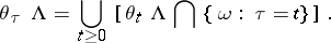
| + | Suppose that, on a measurable space <img align="absmiddle" border="0" src="https://www.encyclopediaofmath.org/legacyimages/m/m062/m062490/m062490143.png" />, a Markov process <img align="absmiddle" border="0" src="https://www.encyclopediaofmath.org/legacyimages/m/m062/m062490/m062490144.png" /> is given. A function <img align="absmiddle" border="0" src="https://www.encyclopediaofmath.org/legacyimages/m/m062/m062490/m062490145.png" /> is called a [[Markov moment|Markov moment]] (stopping time) if <img align="absmiddle" border="0" src="https://www.encyclopediaofmath.org/legacyimages/m/m062/m062490/m062490146.png" /> for <img align="absmiddle" border="0" src="https://www.encyclopediaofmath.org/legacyimages/m/m062/m062490/m062490147.png" />. Here a set <img align="absmiddle" border="0" src="https://www.encyclopediaofmath.org/legacyimages/m/m062/m062490/m062490148.png" /> is considered in the family <img align="absmiddle" border="0" src="https://www.encyclopediaofmath.org/legacyimages/m/m062/m062490/m062490149.png" /> if <img align="absmiddle" border="0" src="https://www.encyclopediaofmath.org/legacyimages/m/m062/m062490/m062490150.png" /> for <img align="absmiddle" border="0" src="https://www.encyclopediaofmath.org/legacyimages/m/m062/m062490/m062490151.png" /> (most often <img align="absmiddle" border="0" src="https://www.encyclopediaofmath.org/legacyimages/m/m062/m062490/m062490152.png" /> is interpreted as the family of events connected with the evolution of <img align="absmiddle" border="0" src="https://www.encyclopediaofmath.org/legacyimages/m/m062/m062490/m062490153.png" /> up to time <img align="absmiddle" border="0" src="https://www.encyclopediaofmath.org/legacyimages/m/m062/m062490/m062490154.png" />). For <img align="absmiddle" border="0" src="https://www.encyclopediaofmath.org/legacyimages/m/m062/m062490/m062490155.png" />, set | ||
| + | |||
| + | <table class="eq" style="width:100%;"> <tr><td valign="top" style="width:94%;text-align:center;"><img align="absmiddle" border="0" src="https://www.encyclopediaofmath.org/legacyimages/m/m062/m062490/m062490156.png" /></td> </tr></table> | ||
| + | |||
| + | A progressively-measurable Markov process <img align="absmiddle" border="0" src="https://www.encyclopediaofmath.org/legacyimages/m/m062/m062490/m062490157.png" /> is called a strong Markov process if for any Markov moment <img align="absmiddle" border="0" src="https://www.encyclopediaofmath.org/legacyimages/m/m062/m062490/m062490158.png" /> and all <img align="absmiddle" border="0" src="https://www.encyclopediaofmath.org/legacyimages/m/m062/m062490/m062490159.png" />, <img align="absmiddle" border="0" src="https://www.encyclopediaofmath.org/legacyimages/m/m062/m062490/m062490160.png" /> and <img align="absmiddle" border="0" src="https://www.encyclopediaofmath.org/legacyimages/m/m062/m062490/m062490161.png" />, the relation | ||
| + | |||
| + | <table class="eq" style="width:100%;"> <tr><td valign="top" style="width:94%;text-align:center;"><img align="absmiddle" border="0" src="https://www.encyclopediaofmath.org/legacyimages/m/m062/m062490/m062490162.png" /></td> <td valign="top" style="width:5%;text-align:right;">(5)</td></tr></table> | ||
| + | |||
| + | (the strong Markov property) is satisfied <img align="absmiddle" border="0" src="https://www.encyclopediaofmath.org/legacyimages/m/m062/m062490/m062490163.png" />-almost certainly in <img align="absmiddle" border="0" src="https://www.encyclopediaofmath.org/legacyimages/m/m062/m062490/m062490164.png" />. In the verification of (5) it suffices to consider only sets of the form <img align="absmiddle" border="0" src="https://www.encyclopediaofmath.org/legacyimages/m/m062/m062490/m062490165.png" /> where <img align="absmiddle" border="0" src="https://www.encyclopediaofmath.org/legacyimages/m/m062/m062490/m062490166.png" />, <img align="absmiddle" border="0" src="https://www.encyclopediaofmath.org/legacyimages/m/m062/m062490/m062490167.png" />; in this case <img align="absmiddle" border="0" src="https://www.encyclopediaofmath.org/legacyimages/m/m062/m062490/m062490168.png" />. For example, any right-continuous Feller–Markov process on a topological space <img align="absmiddle" border="0" src="https://www.encyclopediaofmath.org/legacyimages/m/m062/m062490/m062490169.png" /> is a strong Markov process. A Markov process is called a Feller–Markov process if the function | ||
| + | |||
| + | <table class="eq" style="width:100%;"> <tr><td valign="top" style="width:94%;text-align:center;"><img align="absmiddle" border="0" src="https://www.encyclopediaofmath.org/legacyimages/m/m062/m062490/m062490170.png" /></td> </tr></table> | ||
| + | |||
| + | is continuous whenever <img align="absmiddle" border="0" src="https://www.encyclopediaofmath.org/legacyimages/m/m062/m062490/m062490171.png" /> is continuous and bounded. | ||
| + | |||
| + | In the case of strong Markov processes various subclasses have been distinguished. Let the Markov transition function <img align="absmiddle" border="0" src="https://www.encyclopediaofmath.org/legacyimages/m/m062/m062490/m062490172.png" />, given on a locally compact metric space <img align="absmiddle" border="0" src="https://www.encyclopediaofmath.org/legacyimages/m/m062/m062490/m062490173.png" />, be stochastically continuous: | ||
| + | |||
| + | <table class="eq" style="width:100%;"> <tr><td valign="top" style="width:94%;text-align:center;"><img align="absmiddle" border="0" src="https://www.encyclopediaofmath.org/legacyimages/m/m062/m062490/m062490174.png" /></td> </tr></table> | ||
| + | |||
| + | for any neighbourhood <img align="absmiddle" border="0" src="https://www.encyclopediaofmath.org/legacyimages/m/m062/m062490/m062490175.png" /> of each point <img align="absmiddle" border="0" src="https://www.encyclopediaofmath.org/legacyimages/m/m062/m062490/m062490176.png" />. If <img align="absmiddle" border="0" src="https://www.encyclopediaofmath.org/legacyimages/m/m062/m062490/m062490177.png" /> maps the class of continuous functions that vanish at infinity into itself, then <img align="absmiddle" border="0" src="https://www.encyclopediaofmath.org/legacyimages/m/m062/m062490/m062490178.png" /> corresponds to a standard Markov process <img align="absmiddle" border="0" src="https://www.encyclopediaofmath.org/legacyimages/m/m062/m062490/m062490179.png" />. That is, a right-continuous strong Markov process for which: 1) <img align="absmiddle" border="0" src="https://www.encyclopediaofmath.org/legacyimages/m/m062/m062490/m062490180.png" /> for <img align="absmiddle" border="0" src="https://www.encyclopediaofmath.org/legacyimages/m/m062/m062490/m062490181.png" /> and <img align="absmiddle" border="0" src="https://www.encyclopediaofmath.org/legacyimages/m/m062/m062490/m062490182.png" /> for <img align="absmiddle" border="0" src="https://www.encyclopediaofmath.org/legacyimages/m/m062/m062490/m062490183.png" />; 2) <img align="absmiddle" border="0" src="https://www.encyclopediaofmath.org/legacyimages/m/m062/m062490/m062490184.png" />, <img align="absmiddle" border="0" src="https://www.encyclopediaofmath.org/legacyimages/m/m062/m062490/m062490185.png" />-almost certainly on the set <img align="absmiddle" border="0" src="https://www.encyclopediaofmath.org/legacyimages/m/m062/m062490/m062490186.png" />, where <img align="absmiddle" border="0" src="https://www.encyclopediaofmath.org/legacyimages/m/m062/m062490/m062490187.png" /> and <img align="absmiddle" border="0" src="https://www.encyclopediaofmath.org/legacyimages/m/m062/m062490/m062490188.png" /> (<img align="absmiddle" border="0" src="https://www.encyclopediaofmath.org/legacyimages/m/m062/m062490/m062490189.png" />) are Markov moments that are non-decreasing as <img align="absmiddle" border="0" src="https://www.encyclopediaofmath.org/legacyimages/m/m062/m062490/m062490190.png" /> increases. | ||
| + | |||
| + | ==Terminating Markov processes.== | ||
| + | Frequently, a physical system can be best described using a non-terminating Markov process, but only in a time interval of random length. In addition, even simple transformations of a Markov process may lead to processes with trajectories given on random intervals (see [[Functional of a Markov process|Functional of a Markov process]]). Guided by these considerations one introduces the notion of a terminating Markov process. | ||
| + | |||
| + | Let <img align="absmiddle" border="0" src="https://www.encyclopediaofmath.org/legacyimages/m/m062/m062490/m062490191.png" /> be a homogeneous Markov process in a phase space <img align="absmiddle" border="0" src="https://www.encyclopediaofmath.org/legacyimages/m/m062/m062490/m062490192.png" />, having a transition function <img align="absmiddle" border="0" src="https://www.encyclopediaofmath.org/legacyimages/m/m062/m062490/m062490193.png" />, and let there be a point <img align="absmiddle" border="0" src="https://www.encyclopediaofmath.org/legacyimages/m/m062/m062490/m062490194.png" /> and a function <img align="absmiddle" border="0" src="https://www.encyclopediaofmath.org/legacyimages/m/m062/m062490/m062490195.png" /> such that <img align="absmiddle" border="0" src="https://www.encyclopediaofmath.org/legacyimages/m/m062/m062490/m062490196.png" /> for <img align="absmiddle" border="0" src="https://www.encyclopediaofmath.org/legacyimages/m/m062/m062490/m062490197.png" /> and <img align="absmiddle" border="0" src="https://www.encyclopediaofmath.org/legacyimages/m/m062/m062490/m062490198.png" /> otherwise (unless stated otherwise, take <img align="absmiddle" border="0" src="https://www.encyclopediaofmath.org/legacyimages/m/m062/m062490/m062490199.png" />). A new trajectory <img align="absmiddle" border="0" src="https://www.encyclopediaofmath.org/legacyimages/m/m062/m062490/m062490200.png" /> is given for <img align="absmiddle" border="0" src="https://www.encyclopediaofmath.org/legacyimages/m/m062/m062490/m062490201.png" /> by the equality <img align="absmiddle" border="0" src="https://www.encyclopediaofmath.org/legacyimages/m/m062/m062490/m062490202.png" />, and <img align="absmiddle" border="0" src="https://www.encyclopediaofmath.org/legacyimages/m/m062/m062490/m062490203.png" /> is defined as the trace of <img align="absmiddle" border="0" src="https://www.encyclopediaofmath.org/legacyimages/m/m062/m062490/m062490204.png" /> on the set <img align="absmiddle" border="0" src="https://www.encyclopediaofmath.org/legacyimages/m/m062/m062490/m062490205.png" />. | ||
| + | |||
| + | The collection <img align="absmiddle" border="0" src="https://www.encyclopediaofmath.org/legacyimages/m/m062/m062490/m062490206.png" />, where <img align="absmiddle" border="0" src="https://www.encyclopediaofmath.org/legacyimages/m/m062/m062490/m062490207.png" />, is called the terminating Markov process obtained from <img align="absmiddle" border="0" src="https://www.encyclopediaofmath.org/legacyimages/m/m062/m062490/m062490208.png" /> by censoring (or killing) at the time <img align="absmiddle" border="0" src="https://www.encyclopediaofmath.org/legacyimages/m/m062/m062490/m062490209.png" />. The variable <img align="absmiddle" border="0" src="https://www.encyclopediaofmath.org/legacyimages/m/m062/m062490/m062490210.png" /> is called the censoring time or lifetime of the terminating Markov process. The phase space of the new process is <img align="absmiddle" border="0" src="https://www.encyclopediaofmath.org/legacyimages/m/m062/m062490/m062490211.png" />, where <img align="absmiddle" border="0" src="https://www.encyclopediaofmath.org/legacyimages/m/m062/m062490/m062490212.png" /> is the trace of the <img align="absmiddle" border="0" src="https://www.encyclopediaofmath.org/legacyimages/m/m062/m062490/m062490213.png" />-algebra <img align="absmiddle" border="0" src="https://www.encyclopediaofmath.org/legacyimages/m/m062/m062490/m062490214.png" /> in <img align="absmiddle" border="0" src="https://www.encyclopediaofmath.org/legacyimages/m/m062/m062490/m062490215.png" />. The transition function of a terminating Markov process is the restriction of <img align="absmiddle" border="0" src="https://www.encyclopediaofmath.org/legacyimages/m/m062/m062490/m062490216.png" /> to the set <img align="absmiddle" border="0" src="https://www.encyclopediaofmath.org/legacyimages/m/m062/m062490/m062490217.png" />, <img align="absmiddle" border="0" src="https://www.encyclopediaofmath.org/legacyimages/m/m062/m062490/m062490218.png" />, <img align="absmiddle" border="0" src="https://www.encyclopediaofmath.org/legacyimages/m/m062/m062490/m062490219.png" />. The process <img align="absmiddle" border="0" src="https://www.encyclopediaofmath.org/legacyimages/m/m062/m062490/m062490220.png" /> is called a strong Markov process or a standard Markov process if <img align="absmiddle" border="0" src="https://www.encyclopediaofmath.org/legacyimages/m/m062/m062490/m062490221.png" /> has the corresponding property. A non-terminating Markov process can be considered as a terminating Markov process with censoring time <img align="absmiddle" border="0" src="https://www.encyclopediaofmath.org/legacyimages/m/m062/m062490/m062490222.png" />. A non-homogeneous terminating Markov process is defined similarly. | ||
| + | |||
| + | ''M.G. Shur'' | ||
| + | |||
| + | ==Markov processes and differential equations.== | ||
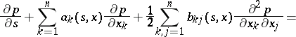
| + | A Markov process of Brownian-motion type is closely connected with partial differential equations of parabolic type. The transition density <img align="absmiddle" border="0" src="https://www.encyclopediaofmath.org/legacyimages/m/m062/m062490/m062490223.png" /> of a diffusion process satisfies, under certain additional assumptions, the backward and forward Kolmogorov equations (cf. [[Kolmogorov equation|Kolmogorov equation]]): | ||
| + | |||
| + | <table class="eq" style="width:100%;"> <tr><td valign="top" style="width:94%;text-align:center;"><img align="absmiddle" border="0" src="https://www.encyclopediaofmath.org/legacyimages/m/m062/m062490/m062490224.png" /></td> <td valign="top" style="width:5%;text-align:right;">(6)</td></tr></table> | ||
| + | |||
| + | <table class="eq" style="width:100%;"> <tr><td valign="top" style="width:94%;text-align:center;"><img align="absmiddle" border="0" src="https://www.encyclopediaofmath.org/legacyimages/m/m062/m062490/m062490225.png" /></td> </tr></table> | ||
| + | |||
| + | <table class="eq" style="width:100%;"> <tr><td valign="top" style="width:94%;text-align:center;"><img align="absmiddle" border="0" src="https://www.encyclopediaofmath.org/legacyimages/m/m062/m062490/m062490226.png" /></td> <td valign="top" style="width:5%;text-align:right;">(7)</td></tr></table> | ||
| + | |||
| + | <table class="eq" style="width:100%;"> <tr><td valign="top" style="width:94%;text-align:center;"><img align="absmiddle" border="0" src="https://www.encyclopediaofmath.org/legacyimages/m/m062/m062490/m062490227.png" /></td> </tr></table> | ||
| + | |||
| + | The function <img align="absmiddle" border="0" src="https://www.encyclopediaofmath.org/legacyimages/m/m062/m062490/m062490228.png" /> is the Green's function of the equations (6)–(7), and the first known methods for constructing diffusion processes were based on existence theorems for this function for the partial differential equations (6)–(7). For a time-homogeneous process the operator <img align="absmiddle" border="0" src="https://www.encyclopediaofmath.org/legacyimages/m/m062/m062490/m062490229.png" /> coincides on smooth functions with the infinitesimal operator of the Markov process (see [[Transition-operator semi-group|Transition-operator semi-group]]). | ||
| + | |||
| + | The expectations of various functionals of diffusion processes are solutions of boundary value problems for the differential equation . Let <img align="absmiddle" border="0" src="https://www.encyclopediaofmath.org/legacyimages/m/m062/m062490/m062490230.png" /> be the expectation with respect to the measure <img align="absmiddle" border="0" src="https://www.encyclopediaofmath.org/legacyimages/m/m062/m062490/m062490231.png" />. Then the function <img align="absmiddle" border="0" src="https://www.encyclopediaofmath.org/legacyimages/m/m062/m062490/m062490232.png" /> satisfies (6) for <img align="absmiddle" border="0" src="https://www.encyclopediaofmath.org/legacyimages/m/m062/m062490/m062490233.png" /> and <img align="absmiddle" border="0" src="https://www.encyclopediaofmath.org/legacyimages/m/m062/m062490/m062490234.png" />. | ||
| + | |||
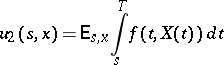
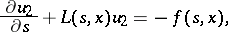
| + | Similarly, the function | ||
| + | |||
| + | <table class="eq" style="width:100%;"> <tr><td valign="top" style="width:94%;text-align:center;"><img align="absmiddle" border="0" src="https://www.encyclopediaofmath.org/legacyimages/m/m062/m062490/m062490235.png" /></td> </tr></table> | ||
| + | |||
| + | satisfies, for <img align="absmiddle" border="0" src="https://www.encyclopediaofmath.org/legacyimages/m/m062/m062490/m062490236.png" />, | ||
| + | |||
| + | <table class="eq" style="width:100%;"> <tr><td valign="top" style="width:94%;text-align:center;"><img align="absmiddle" border="0" src="https://www.encyclopediaofmath.org/legacyimages/m/m062/m062490/m062490237.png" /></td> </tr></table> | ||
| + | |||
| + | and <img align="absmiddle" border="0" src="https://www.encyclopediaofmath.org/legacyimages/m/m062/m062490/m062490238.png" />. | ||
| + | |||
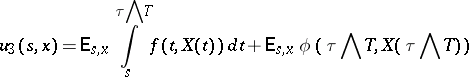
| + | Let <img align="absmiddle" border="0" src="https://www.encyclopediaofmath.org/legacyimages/m/m062/m062490/m062490239.png" /> be the time at which the trajectories of <img align="absmiddle" border="0" src="https://www.encyclopediaofmath.org/legacyimages/m/m062/m062490/m062490240.png" /> first hit the boundary <img align="absmiddle" border="0" src="https://www.encyclopediaofmath.org/legacyimages/m/m062/m062490/m062490241.png" /> of a domain <img align="absmiddle" border="0" src="https://www.encyclopediaofmath.org/legacyimages/m/m062/m062490/m062490242.png" />, and let <img align="absmiddle" border="0" src="https://www.encyclopediaofmath.org/legacyimages/m/m062/m062490/m062490243.png" />. Then, under certain conditions, the function | ||
| + | |||
| + | <table class="eq" style="width:100%;"> <tr><td valign="top" style="width:94%;text-align:center;"><img align="absmiddle" border="0" src="https://www.encyclopediaofmath.org/legacyimages/m/m062/m062490/m062490244.png" /></td> </tr></table> | ||
| + | |||
| + | satisfies | ||
| + | |||
| + | <table class="eq" style="width:100%;"> <tr><td valign="top" style="width:94%;text-align:center;"><img align="absmiddle" border="0" src="https://www.encyclopediaofmath.org/legacyimages/m/m062/m062490/m062490245.png" /></td> </tr></table> | ||
| + | |||
| + | and takes the value <img align="absmiddle" border="0" src="https://www.encyclopediaofmath.org/legacyimages/m/m062/m062490/m062490246.png" /> on the set | ||
| + | |||
| + | <table class="eq" style="width:100%;"> <tr><td valign="top" style="width:94%;text-align:center;"><img align="absmiddle" border="0" src="https://www.encyclopediaofmath.org/legacyimages/m/m062/m062490/m062490247.png" /></td> </tr></table> | ||
| + | |||
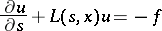
| + | The solution of the first boundary value problem for a general second-order linear parabolic equation | ||
| + | |||
| + | <table class="eq" style="width:100%;"> <tr><td valign="top" style="width:94%;text-align:center;"><img align="absmiddle" border="0" src="https://www.encyclopediaofmath.org/legacyimages/m/m062/m062490/m062490248.png" /></td> <td valign="top" style="width:5%;text-align:right;">(8)</td></tr></table> | ||
| + | |||
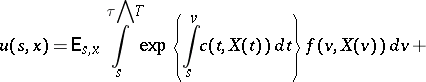
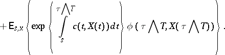
| + | can, under fairly general assumptions, be described in the form | ||
| + | |||
| + | <table class="eq" style="width:100%;"> <tr><td valign="top" style="width:94%;text-align:center;"><img align="absmiddle" border="0" src="https://www.encyclopediaofmath.org/legacyimages/m/m062/m062490/m062490249.png" /></td> <td valign="top" style="width:5%;text-align:right;">(9)</td></tr></table> | ||
| + | |||
| + | <table class="eq" style="width:100%;"> <tr><td valign="top" style="width:94%;text-align:center;"><img align="absmiddle" border="0" src="https://www.encyclopediaofmath.org/legacyimages/m/m062/m062490/m062490250.png" /></td> </tr></table> | ||
| + | |||
| + | When the operator <img align="absmiddle" border="0" src="https://www.encyclopediaofmath.org/legacyimages/m/m062/m062490/m062490251.png" /> and the functions <img align="absmiddle" border="0" src="https://www.encyclopediaofmath.org/legacyimages/m/m062/m062490/m062490252.png" /> and <img align="absmiddle" border="0" src="https://www.encyclopediaofmath.org/legacyimages/m/m062/m062490/m062490253.png" /> do not depend on <img align="absmiddle" border="0" src="https://www.encyclopediaofmath.org/legacyimages/m/m062/m062490/m062490254.png" />, a representation similar to (9) is possible also for the solution of a linear elliptic equation. More precisely, the function | ||
| + | |||
| + | <table class="eq" style="width:100%;"> <tr><td valign="top" style="width:94%;text-align:center;"><img align="absmiddle" border="0" src="https://www.encyclopediaofmath.org/legacyimages/m/m062/m062490/m062490255.png" /></td> <td valign="top" style="width:5%;text-align:right;">(10)</td></tr></table> | ||
| + | |||
| + | <table class="eq" style="width:100%;"> <tr><td valign="top" style="width:94%;text-align:center;"><img align="absmiddle" border="0" src="https://www.encyclopediaofmath.org/legacyimages/m/m062/m062490/m062490256.png" /></td> </tr></table> | ||
| + | |||
| + | is, under certain assumptions, the solution of | ||
| + | |||
| + | <table class="eq" style="width:100%;"> <tr><td valign="top" style="width:94%;text-align:center;"><img align="absmiddle" border="0" src="https://www.encyclopediaofmath.org/legacyimages/m/m062/m062490/m062490257.png" /></td> <td valign="top" style="width:5%;text-align:right;">(11)</td></tr></table> | ||
| + | |||
| + | When <img align="absmiddle" border="0" src="https://www.encyclopediaofmath.org/legacyimages/m/m062/m062490/m062490258.png" /> is degenerate <img align="absmiddle" border="0" src="https://www.encyclopediaofmath.org/legacyimages/m/m062/m062490/m062490259.png" /> or <img align="absmiddle" border="0" src="https://www.encyclopediaofmath.org/legacyimages/m/m062/m062490/m062490260.png" /> is not sufficiently "smooth" , the boundary values need not be taken by the functions (9), (10) at individual points or on whole sets. The notion of a [[Regular boundary point|regular boundary point]] for <img align="absmiddle" border="0" src="https://www.encyclopediaofmath.org/legacyimages/m/m062/m062490/m062490261.png" /> has a probabilistic interpretation. At regular points the boundary values are attained by (9), (10). The solution of (8) and (11) allows one to study the properties of the corresponding diffusion processes and functionals of them. | ||
| + | |||
| + | There are methods for constructing Markov processes which do not rely on the construction of solutions of (6) and (7). For example, the method of stochastic differential equations (cf. [[Stochastic differential equation|Stochastic differential equation]]), of absolutely-continuous change of measure, etc. This situation, together with the formulas (9) and (10), gives a probabilistic route to the construction and study of the properties of boundary value problems for (8) and also to the study of properties of the solutions of the corresponding elliptic equation. | ||
| + | |||
| + | Since the solution of a stochastic differential equation is insensitive to degeneracy of <img align="absmiddle" border="0" src="https://www.encyclopediaofmath.org/legacyimages/m/m062/m062490/m062490262.png" />, probabilistic methods can be applied to construct solutions of degenerate elliptic and parabolic differential equations. The extension of the averaging principle of N.M. Krylov and N.N. Bogolyubov to stochastic differential equations allows one, with the help of (9), to obtain corresponding results for elliptic and parabolic differential equations. It turns out that certain difficult problems in the investigation of properties of solutions of equations of this type with small parameters in front of the highest derivatives can be solved by probabilistic arguments. Even the solution of the second boundary value problem for (6) has a probabilistic meaning. The formulation of boundary value problems for unbounded domains is closely connected with recurrence in the corresponding diffusion process. | ||
| + | |||
| + | In the case of a time-homogeneous process (<img align="absmiddle" border="0" src="https://www.encyclopediaofmath.org/legacyimages/m/m062/m062490/m062490263.png" /> is independent of <img align="absmiddle" border="0" src="https://www.encyclopediaofmath.org/legacyimages/m/m062/m062490/m062490264.png" />), a positive solution of <img align="absmiddle" border="0" src="https://www.encyclopediaofmath.org/legacyimages/m/m062/m062490/m062490265.png" /> coincides, under certain assumptions and up to a multiplicative constant, with the stationary density of the distribution of a Markov chain. Probabilistic arguments turn out to be useful even for boundary value problems for non-linear parabolic equations. | ||
| + | |||
| + | ''R.Z. Khas'minskii'' | ||
| + | |||
| + | References to all sections are given below. | ||
| + | |||
| + | ====References==== | ||
| + | {| | ||
| + | |valign="top"|{{Ref|M}}|| A.A. Markov, "?", ''Izv. Fiz.-Mat. Obshch. Kazan. Univ.'' , '''15''' : 4 (1906) pp. 135–156 | ||
| + | |- | ||
| + | |valign="top"|{{Ref|B}}|| L. Bachelier, "?", ''Ann. Sci. Ecole Norm. Sup.'' , '''17''' (1900) pp. 21–86 | ||
| + | |- | ||
| + | |valign="top"|{{Ref|Ko}}|| A.N. Kolmogorov, "Ueber die analytischen Methoden in der Wahrscheinlichkeitsrechnung" ''Math. Ann.'' , '''104''' (1931) pp. 415–458 | ||
| + | |- | ||
| + | |valign="top"|{{Ref|C}}|| K.L. Chung, "Markov chains with stationary transition probabilities" , Springer (1967) {{MR|0217872}} {{ZBL|0146.38401}} | ||
| + | |- | ||
| + | |valign="top"|{{Ref|F}}|| W. Feller, "The general diffusion operator and positivity-preserving semi-groups in one dimension" ''Ann. of Math.'' , '''60''' (1954) pp. 417–436 {{MR|0065809}} {{ZBL|}} | ||
| + | |- | ||
| + | |valign="top"|{{Ref|DY}}|| E.B. Dynkin, A.A. Yushkevich, "Strong Markov processs" ''Theor. Veroyatnost. i Primenen.'' , '''1''' : 1 (1956) pp. 149–155 (In Russian) (English abstract) | ||
| + | |- | ||
| + | |valign="top"|{{Ref|H}}|| G.A. Hunt, "Markov processes and potentials I" ''Illinois J. Math.'' , '''1''' (1957) pp. 44–93 | ||
| + | |- | ||
| + | |valign="top"|{{Ref|H2}}|| G.A. Hunt, "Markov processes and potentials II" ''Illinois J. Math.'' , '''1''' (1957) pp. 316–369 | ||
| + | |- | ||
| + | |valign="top"|{{Ref|H3}}|| G.A. Hunt, "Markov processes and potentials III" ''Illinois J. Math.'' , '''2''' (1958) pp. 151–213 | ||
| + | |- | ||
| + | |valign="top"|{{Ref|De}}|| C. Dellacherie, "Capacités et processus stochastiques" , Springer (1972) {{MR|0448504}} {{ZBL|0246.60032}} | ||
| + | |- | ||
| + | |valign="top"|{{Ref|Dy}}|| E.B. Dynkin, "Theory of Markov processes" , Pergamon (1960) (Translated from Russian) {{MR|2305744}} {{MR|1009436}} {{MR|0245096}} {{MR|1531923}} {{MR|0131900}} {{MR|0131898}} {{ZBL|1116.60001}} {{ZBL|0689.60003}} {{ZBL|0222.60048}} {{ZBL|0091.13605}} | ||
| + | |- | ||
| + | |valign="top"|{{Ref|D2}}|| E.B. Dynkin, "Markov processes" , '''1''' , Springer (1965) (Translated from Russian) {{MR|0193671}} {{ZBL|0132.37901}} | ||
| + | |- | ||
| + | |valign="top"|{{Ref|GS}}|| I.I. Gihman, A.V. Skorohod, "The theory of stochastic processes" , '''2''' , Springer (1979) (Translated from Russian) {{MR|0651014}} {{MR|0651015}} {{ZBL|0404.60061}} | ||
| + | |- | ||
| + | |valign="top"|{{Ref|Fr}}|| M.I. Freidlin, "Markov processes and differential equations" ''Itogi Nauk. Teor. Veroyatnost. Mat. Statist. Teoret. Kibernet. 1966'' (1967) pp. 7–58 (In Russian) {{MR|0235308}} {{ZBL|0863.60049}} | ||
| + | |- | ||
| + | |valign="top"|{{Ref|Kh}}|| R.Z. Khas'minskii, "Principle of averaging for parabolic and elliptic partial differential equations and for Markov processes with small diffusion" ''Theor. Probab. Appl.'' , '''8''' (1963) pp. 1–21 ''Teor. Veroyatnost. i Primenen.'' , '''8''' : 1 (1963) pp. 3–25 | ||
| + | |- | ||
| + | |valign="top"|{{Ref|VF}}|| A.D. Venttsel', M.I. Freidlin, "Random perturbations of dynamical systems" , Springer (1984) (Translated from Russian) {{MR|722136}} {{ZBL|}} | ||
| + | |- | ||
| + | |valign="top"|{{Ref|BG}}|| R.M. Blumenthal, R.K. Getoor, "Markov processes and potential theory" , Acad. Press (1968) {{MR|0264757}} {{ZBL|0169.49204}} | ||
| + | |- | ||
| + | |valign="top"|{{Ref|G}}|| R.K. Getoor, "Markov processes: Ray processes and right processes" , ''Lect. notes in math.'' , '''440''' , Springer (1975) {{MR|0405598}} {{ZBL|0299.60051}} | ||
| + | |- | ||
| + | |valign="top"|{{Ref|Kuz}}|| S.E. Kuznetsov, "Any Markov process in a Borel space has a transition function" ''Theor. Prob. Appl.'' , '''25''' (1980) pp. 384–388 ''Teor. Veroyatnost. i Primenen.'' , '''25''' : 2 (1980) pp. 389–393 {{MR|0572574}} {{ZBL|0456.60077}} {{ZBL|0431.60071}} | ||
| + | |} | ||
| + | |||
| + | ====Comments==== | ||
| + | |||
| + | |||
| + | ====References==== | ||
| + | {| | ||
| + | |valign="top"|{{Ref|SV}}|| D.W. Stroock, S.R.S. Varadhan, "Multidimensional diffusion processes" , Springer (1979) {{MR|0532498}} {{ZBL|0426.60069}} | ||
| + | |- | ||
| + | |valign="top"|{{Ref|C2}}|| K.L. Chung, "Lectures from Markov processes to Brownian motion" , Springer (1982) {{MR|0648601}} {{ZBL|0503.60073}} | ||
| + | |- | ||
| + | |valign="top"|{{Ref|Do}}|| J.L. Doob, "Stochastic processes" , Wiley (1953) {{MR|1570654}} {{MR|0058896}} {{ZBL|0053.26802}} | ||
| + | |- | ||
| + | |valign="top"|{{Ref|We}}|| A.D. Wentzell, "A course in the theory of stochastic processes" , McGraw-Hill (1981) (Translated from Russian) {{MR|0781738}} {{MR|0614594}} {{ZBL|0502.60001}} | ||
| + | |- | ||
| + | |valign="top"|{{Ref|Kur}}|| T.G. Kurtz, "Markov processes" , Wiley (1986) {{MR|0838085}} {{ZBL|0592.60049}} | ||
| + | |- | ||
| + | |valign="top"|{{Ref|F2}}|| W. Feller, "An introduction to probability theory and its applications" , '''1–2''' , Wiley (1966) {{MR|0210154}} {{ZBL|0138.10207}} | ||
| + | |- | ||
| + | |valign="top"|{{Ref|Wa}}|| N. Wax (ed.), ''Selected papers on noise and stochastic processes'' , Dover, reprint (1954) {{MR|}} {{ZBL|0059.11903}} | ||
| + | |- | ||
| + | |valign="top"|{{Ref|Ka}}|| M. Kac, "Probability and related topics in physical sciences" , Interscience (1959) pp. Chapt. 4 {{MR|0102849}} {{ZBL|0087.33003}} | ||
| + | |- | ||
| + | |valign="top"|{{Ref|Le}}|| P. Lévy, "Processus stochastiques et mouvement Brownien" , Gauthier-Villars (1965) {{MR|0190953}} {{ZBL|0137.11602}} | ||
| + | |- | ||
| + | |valign="top"|{{Ref|Lo}}|| M. Loève, "Probability theory" , '''II''' , Springer (1978) {{MR|0651017}} {{MR|0651018}} {{ZBL|0385.60001}} | ||
| + | |} | ||
Revision as of 23:22, 13 March 2016
process without after-effects
2020 Mathematics Subject Classification: Primary: 60Jxx [MSN][ZBL]
A stochastic process whose evolution after a given time  does not depend on the evolution before
  , given that the value of the process at
  is fixed (briefly; the "future" and "past" of the process are independent of each other for a known "present" ).
The defining property of a Markov process is commonly called the Markov property; it was first stated by A.A. Markov . However, in the work of L. Bachelier it is already possible to find an attempt to discuss Brownian motion as a Markov process, an attempt which received justification later in the research of N. Wiener (1923). The basis of the general theory of continuous-time Markov processes was laid by A.N. Kolmogorov .
The Markov property.
There are essentially distinct definitions of a Markov process. One of the more widely used is the following. On a probability space  let there be given a stochastic process
  ,
,  , taking values in a measurable space
  , where
  is a subset of the real line
  . Let
. Let  (respectively,
  ) be the
  -algebra in
  generated by the variables
  for
for  (
( ), where
  . In other words,
  (respectively,
  ) is the collection of events connected with the evolution of the process up to time (starting from time)
  .
.  is called a Markov process if (almost certainly) for all
  ,
,  the Markov property
 | (1) |
holds, or, what is the same, if for any  and
and  ,
,
 | (2) |
A Markov process for which  is contained in the natural numbers is called a Markov chain (however, the latter term is mostly associated with the case of an at most countable
  ). If
). If  is an interval in
  and
and  is at most countable, a Markov process is called a continuous-time Markov chain. Examples of continuous-time Markov processes are furnished by diffusion processes (cf. Diffusion process) and processes with independent increments (cf. Stochastic process with independent increments), including Poisson and Wiener processes (cf. Poisson process; Wiener process).
In what follows the discussion will concern only the case  , for the sake of being specific. The formulas (1) and (2) give an explicit interpretation of the principle of independence of "past" and "future" events when the "present" is known, but the definition of Markov process based on them has proved to be insufficiently flexible in the numerous situations where one is obliged to consider not one, but a collection of conditions of the type (1) or (2) corresponding to different, but in some sense consistent, measures
  . Such reasoning has led to the acceptance of the following definitions (see , ).
Suppose one is given:
a) a measurable space  , where the
  -algebra
  contains all one-point sets in
  ;
;
b) a measurable space  , equipped with a family of
  -algebras
  ,
,  , such that
  if
if  ;
;
c) a function ( "trajectory" )  , defining for
  and
and  a measurable mapping from
  to
to  ;
;
d) for each  and
and  a probability measure
  on the
  -algebra
  such that the function
  is measurable with respect to
  , if
, if  and
and  .
.
The collection 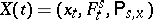 is called a (non-terminating) Markov process given on
  if
if  -almost certainly
 | (3) |
for any  and
and  . Here
  is the space of elementary events,
  is the phase space or state space and
  is the transition function or transition probability of
  . If
. If  is endowed with a topology and
  is the collection of Borel sets in
  , then it is commonly said that the Markov process is given on
  . Usually included in the definition of a Markov process is the requirement that
  , and then
  ,
,  , is interpreted as the probability of
  under the condition that
  .
.
The following question arises: Is every Markov transition function  , given on a measurable space
  , the transition function of some Markov process? The answer is affirmative if, for example,
  is a separable, locally compact space and
  is the family of Borel sets in
  . In addition, let
  be a complete metric space and let
 |
for any  , where
 |
and  is the complement of the
  -neighbourhood of
  . Then the corresponding Markov process can be taken to be right-continuous and having left limits (that is, its trajectories can be chosen so). The existence of a continuous Markov process is guaranteed by the condition
  as
as  (see , ).
In the theory of Markov processes most attention is given to homogeneous (in time) processes. The corresponding definition assumes one is given a system of objects a)–d) with the difference that the parameters  and
and  may now only take the value 0. Even the notation can be simplified:
 |
 |
Subsequently, homogeneity of  is assumed. That is, it is required that for any
  and
and  there is an
  such that
  for
for  . Because of this, on the
  -algebra
  , the smallest
  -algebra in
  containing the events
  , the time shift operators
  are defined, which preserve the operations of union, intersection and difference of sets, and for which
 |
where  ,
,  .
.
The collection  is called a (non-terminating) homogeneous Markov process given on
  if
if  -almost certainly
 | (4) |
for  ,
,  and
and  . The transition function of
  is taken to be
  , where, unless otherwise indicated, it is required that
  . It is useful to bear in mind that in the verification of (4) it is only necessary to consider sets of the form
  , where
  ,
,  , and in (4),
  may always replaced by the
  -algebra
  equal to the intersection of the completions of
  relative to all possible measures
  . Often, one fixes on
  a probability measure
  (the "initial distribution" ) and considers a random Markov function
  , where
  is the measure on
  given by
 |
A Markov process  is called progressively measurable if for each
  the function
  induces a measurable mapping from
  to
to  , where
  is the
  -algebra of Borel subsets of
  . A right-continuous Markov process is progressively measurable. There is a method for reducing the non-homogeneous case to the homogeneous case (see ), and in what follows homogeneous Markov processes will be discussed.
The strong Markov property.
Suppose that, on a measurable space  , a Markov process
  is given. A function
  is called a Markov moment (stopping time) if
  for
for  . Here a set
  is considered in the family
  if
if  for
for  (most often
  is interpreted as the family of events connected with the evolution of
  up to time
  ). For
  , set
, set
 |
A progressively-measurable Markov process  is called a strong Markov process if for any Markov moment
  and all
  ,
,  and
and  , the relation
 | (5) |
(the strong Markov property) is satisfied  -almost certainly in
  . In the verification of (5) it suffices to consider only sets of the form
  where
where  ,
,  ; in this case
  . For example, any right-continuous Feller–Markov process on a topological space
  is a strong Markov process. A Markov process is called a Feller–Markov process if the function
 |
is continuous whenever  is continuous and bounded.
In the case of strong Markov processes various subclasses have been distinguished. Let the Markov transition function  , given on a locally compact metric space
  , be stochastically continuous:
 |
for any neighbourhood  of each point
  . If
. If  maps the class of continuous functions that vanish at infinity into itself, then
  corresponds to a standard Markov process
  . That is, a right-continuous strong Markov process for which: 1)
  for
for  and
and  for
for  ; 2)
; 2)  ,
,  -almost certainly on the set
  , where
  and
and  (
( ) are Markov moments that are non-decreasing as
  increases.
Terminating Markov processes.
Frequently, a physical system can be best described using a non-terminating Markov process, but only in a time interval of random length. In addition, even simple transformations of a Markov process may lead to processes with trajectories given on random intervals (see Functional of a Markov process). Guided by these considerations one introduces the notion of a terminating Markov process.
Let  be a homogeneous Markov process in a phase space
  , having a transition function
  , and let there be a point
  and a function
  such that
  for
for  and
and  otherwise (unless stated otherwise, take
  ). A new trajectory
  is given for
  by the equality
  , and
, and  is defined as the trace of
  on the set
  .
.
The collection  , where
 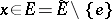 , is called the terminating Markov process obtained from
  by censoring (or killing) at the time
  . The variable
  is called the censoring time or lifetime of the terminating Markov process. The phase space of the new process is
  , where
  is the trace of the
  -algebra
  in
in  . The transition function of a terminating Markov process is the restriction of
  to the set
  ,
,  ,
,  . The process
  is called a strong Markov process or a standard Markov process if
  has the corresponding property. A non-terminating Markov process can be considered as a terminating Markov process with censoring time
  . A non-homogeneous terminating Markov process is defined similarly.
M.G. Shur
Markov processes and differential equations.
A Markov process of Brownian-motion type is closely connected with partial differential equations of parabolic type. The transition density  of a diffusion process satisfies, under certain additional assumptions, the backward and forward Kolmogorov equations (cf. Kolmogorov equation):
 | (6) |
 |
 | (7) |
 |
The function  is the Green's function of the equations (6)–(7), and the first known methods for constructing diffusion processes were based on existence theorems for this function for the partial differential equations (6)–(7). For a time-homogeneous process the operator
  coincides on smooth functions with the infinitesimal operator of the Markov process (see Transition-operator semi-group).
The expectations of various functionals of diffusion processes are solutions of boundary value problems for the differential equation . Let  be the expectation with respect to the measure
  . Then the function
  satisfies (6) for
  and
and  .
.
Similarly, the function
 |
satisfies, for  ,
,
 |
and  .
.
Let  be the time at which the trajectories of
  first hit the boundary
  of a domain
  , and let
 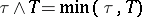 . Then, under certain conditions, the function
 |
satisfies
 |
and takes the value  on the set
 |
The solution of the first boundary value problem for a general second-order linear parabolic equation
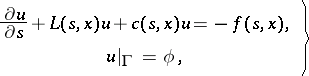 | (8) |
can, under fairly general assumptions, be described in the form
 | (9) |
 |
When the operator  and the functions
  and
and  do not depend on
  , a representation similar to (9) is possible also for the solution of a linear elliptic equation. More precisely, the function
 | (10) |
 |
is, under certain assumptions, the solution of
 | (11) |
When  is degenerate
  or
or  is not sufficiently "smooth" , the boundary values need not be taken by the functions (9), (10) at individual points or on whole sets. The notion of a regular boundary point for
  has a probabilistic interpretation. At regular points the boundary values are attained by (9), (10). The solution of (8) and (11) allows one to study the properties of the corresponding diffusion processes and functionals of them.
There are methods for constructing Markov processes which do not rely on the construction of solutions of (6) and (7). For example, the method of stochastic differential equations (cf. Stochastic differential equation), of absolutely-continuous change of measure, etc. This situation, together with the formulas (9) and (10), gives a probabilistic route to the construction and study of the properties of boundary value problems for (8) and also to the study of properties of the solutions of the corresponding elliptic equation.
Since the solution of a stochastic differential equation is insensitive to degeneracy of  , probabilistic methods can be applied to construct solutions of degenerate elliptic and parabolic differential equations. The extension of the averaging principle of N.M. Krylov and N.N. Bogolyubov to stochastic differential equations allows one, with the help of (9), to obtain corresponding results for elliptic and parabolic differential equations. It turns out that certain difficult problems in the investigation of properties of solutions of equations of this type with small parameters in front of the highest derivatives can be solved by probabilistic arguments. Even the solution of the second boundary value problem for (6) has a probabilistic meaning. The formulation of boundary value problems for unbounded domains is closely connected with recurrence in the corresponding diffusion process.
In the case of a time-homogeneous process ( is independent of
  ), a positive solution of
  coincides, under certain assumptions and up to a multiplicative constant, with the stationary density of the distribution of a Markov chain. Probabilistic arguments turn out to be useful even for boundary value problems for non-linear parabolic equations.
R.Z. Khas'minskii
References to all sections are given below.
References
| [M] | A.A. Markov, "?", Izv. Fiz.-Mat. Obshch. Kazan. Univ. , 15 : 4 (1906) pp. 135–156 |
| [B] | L. Bachelier, "?", Ann. Sci. Ecole Norm. Sup. , 17 (1900) pp. 21–86 |
| [Ko] | A.N. Kolmogorov, "Ueber die analytischen Methoden in der Wahrscheinlichkeitsrechnung" Math. Ann. , 104 (1931) pp. 415–458 |
| [C] | K.L. Chung, "Markov chains with stationary transition probabilities" , Springer (1967) MR0217872 Zbl 0146.38401 |
| [F] | W. Feller, "The general diffusion operator and positivity-preserving semi-groups in one dimension" Ann. of Math. , 60 (1954) pp. 417–436 MR0065809 |
| [DY] | E.B. Dynkin, A.A. Yushkevich, "Strong Markov processs" Theor. Veroyatnost. i Primenen. , 1 : 1 (1956) pp. 149–155 (In Russian) (English abstract) |
| [H] | G.A. Hunt, "Markov processes and potentials I" Illinois J. Math. , 1 (1957) pp. 44–93 |
| [H2] | G.A. Hunt, "Markov processes and potentials II" Illinois J. Math. , 1 (1957) pp. 316–369 |
| [H3] | G.A. Hunt, "Markov processes and potentials III" Illinois J. Math. , 2 (1958) pp. 151–213 |
| [De] | C. Dellacherie, "Capacités et processus stochastiques" , Springer (1972) MR0448504 Zbl 0246.60032 |
| [Dy] | E.B. Dynkin, "Theory of Markov processes" , Pergamon (1960) (Translated from Russian) MR2305744 MR1009436 MR0245096 MR1531923 MR0131900 MR0131898 Zbl 1116.60001 Zbl 0689.60003 Zbl 0222.60048 Zbl 0091.13605 |
| [D2] | E.B. Dynkin, "Markov processes" , 1 , Springer (1965) (Translated from Russian) MR0193671 Zbl 0132.37901 |
| [GS] | I.I. Gihman, A.V. Skorohod, "The theory of stochastic processes" , 2 , Springer (1979) (Translated from Russian) MR0651014 MR0651015 Zbl 0404.60061 |
| [Fr] | M.I. Freidlin, "Markov processes and differential equations" Itogi Nauk. Teor. Veroyatnost. Mat. Statist. Teoret. Kibernet. 1966 (1967) pp. 7–58 (In Russian) MR0235308 Zbl 0863.60049 |
| [Kh] | R.Z. Khas'minskii, "Principle of averaging for parabolic and elliptic partial differential equations and for Markov processes with small diffusion" Theor. Probab. Appl. , 8 (1963) pp. 1–21 Teor. Veroyatnost. i Primenen. , 8 : 1 (1963) pp. 3–25 |
| [VF] | A.D. Venttsel', M.I. Freidlin, "Random perturbations of dynamical systems" , Springer (1984) (Translated from Russian) MR722136 |
| [BG] | R.M. Blumenthal, R.K. Getoor, "Markov processes and potential theory" , Acad. Press (1968) MR0264757 Zbl 0169.49204 |
| [G] | R.K. Getoor, "Markov processes: Ray processes and right processes" , Lect. notes in math. , 440 , Springer (1975) MR0405598 Zbl 0299.60051 |
| [Kuz] | S.E. Kuznetsov, "Any Markov process in a Borel space has a transition function" Theor. Prob. Appl. , 25 (1980) pp. 384–388 Teor. Veroyatnost. i Primenen. , 25 : 2 (1980) pp. 389–393 MR0572574 Zbl 0456.60077 Zbl 0431.60071 |
Comments
References
| [SV] | D.W. Stroock, S.R.S. Varadhan, "Multidimensional diffusion processes" , Springer (1979) MR0532498 Zbl 0426.60069 |
| [C2] | K.L. Chung, "Lectures from Markov processes to Brownian motion" , Springer (1982) MR0648601 Zbl 0503.60073 |
| [Do] | J.L. Doob, "Stochastic processes" , Wiley (1953) MR1570654 MR0058896 Zbl 0053.26802 |
| [We] | A.D. Wentzell, "A course in the theory of stochastic processes" , McGraw-Hill (1981) (Translated from Russian) MR0781738 MR0614594 Zbl 0502.60001 |
| [Kur] | T.G. Kurtz, "Markov processes" , Wiley (1986) MR0838085 Zbl 0592.60049 |
| [F2] | W. Feller, "An introduction to probability theory and its applications" , 1–2 , Wiley (1966) MR0210154 Zbl 0138.10207 |
| [Wa] | N. Wax (ed.), Selected papers on noise and stochastic processes , Dover, reprint (1954) Zbl 0059.11903 |
| [Ka] | M. Kac, "Probability and related topics in physical sciences" , Interscience (1959) pp. Chapt. 4 MR0102849 Zbl 0087.33003 |
| [Le] | P. Lévy, "Processus stochastiques et mouvement Brownien" , Gauthier-Villars (1965) MR0190953 Zbl 0137.11602 |
| [Lo] | M. Loève, "Probability theory" , II , Springer (1978) MR0651017 MR0651018 Zbl 0385.60001 |
Markov process. Encyclopedia of Mathematics. URL: http://encyclopediaofmath.org/index.php?title=Markov_process&oldid=37904