Difference between revisions of "M-estimator"
(Importing text file) |
m (AUTOMATIC EDIT (latexlist): Replaced 115 formulas out of 119 by TEX code with an average confidence of 2.0 and a minimal confidence of 2.0.) |
||
| Line 1: | Line 1: | ||
| − | + | <!--This article has been texified automatically. Since there was no Nroff source code for this article, | |
| + | the semi-automatic procedure described at https://encyclopediaofmath.org/wiki/User:Maximilian_Janisch/latexlist | ||
| + | was used. | ||
| + | If the TeX and formula formatting is correct, please remove this message and the {{TEX|semi-auto}} category. | ||
| − | + | Out of 119 formulas, 115 were replaced by TEX code.--> | |
| − | + | {{TEX|semi-auto}}{{TEX|partial}} | |
| + | A generalization of the maximum-likelihood estimator (MLE) in [[Mathematical statistics|mathematical statistics]] (cf. also [[Maximum-likelihood method|Maximum-likelihood method]]; [[Statistical estimator|Statistical estimator]]). Suppose one has univariate observations $x _ { 1 } , \ldots , x _ { n }$ which are independent and identically distributed according to a distribution $F _ { \theta }$ with univariate parameter $\theta$. Denote by $f _ { \theta } ( x )$ the likelihood of $F _ { \theta }$. The maximum-likelihood estimator is defined as the value $T _ { n } = T _ { n } ( x _ { 1 } , \ldots , x _ { n } )$ which maximizes $\prod _ { i = 1 } ^ { n } f _ { T _ { n } } ( x _ { i } )$. If $f _ { \theta } ( x ) > 0$ for all $x$ and $\theta$, then this is equivalent to minimizing $\sum _ { i = 1 } ^ { n } [ - \operatorname { ln } f _ { T _ { n } } ( x _ { i } ) ]$. P.J. Huber [[#References|[a1]]] has generalized this to M-estimators, which are defined by minimizing $\sum _ { i = 1 } ^ { n } \rho ( x _ { i } , T _ { n } )$, where $\rho$ is an arbitrary real function. When $\rho$ has a partial derivative $\Psi ( x , \theta ) = ( \partial / \partial \theta ) \rho ( x , \theta )$, then $T _ { n }$ satisfies the implicit equation | ||
| − | + | \begin{equation*} \sum _ { i = 1 } ^ { n } \Psi ( x _ { i } , T _ { n } ) = 0. \end{equation*} | |
| − | + | Note that the maximum-likelihood estimator is an M-estimator, obtained by putting $\rho ( x , \theta ) = - \operatorname { ln } f _ { \theta } ( x )$. | |
| − | + | The maximum-likelihood estimator can give arbitrarily bad results when the underlying assumptions (e.g., the form of the distribution generating the data) are not satisfied (e.g., because the data contain some outliers, cf. also [[Outlier|Outlier]]). M-estimators are particularly useful in [[Robust statistics|robust statistics]], which aims to construct methods that are relatively insensitive to deviations from the standard assumptions. M-estimators with bounded $\Psi$ are typically robust. | |
| − | + | Apart from the finite-sample version $T _ { n } ( x _ { 1 } , \ldots , x _ { n } )$ of the M-estimator, there is also a functional version $T ( G )$ defined for any [[Probability distribution|probability distribution]] $G$ by | |
| − | + | \begin{equation*} \int \Psi ( x , T ( G ) ) d G ( x ) = 0. \end{equation*} | |
| − | + | Here, it is assumed that $T$ is Fisher-consistent, i.e. that $T ( F _ { \theta } ) = \theta$ for all $\theta$. The influence function of a functional $T$ in $G$ is defined, as in [[#References|[a2]]], by | |
| − | + | \begin{equation*} \operatorname { IF } ( x ; T , G ) = \frac { \partial } { \partial \varepsilon } [ T ( ( 1 - \varepsilon ) G + \varepsilon \Delta _ { x } ) ]_{\varepsilon = 0 +}, \end{equation*} | |
| − | + | where $\Delta _ { x }$ is the probability distribution which puts all its mass in the point $x$. Therefore $\operatorname{IF} ( x ; T , G )$ describes the effect of a single outlier in $x$ on the estimator $T$. For an M-estimator $T$ at $F _ { \theta }$, | |
| − | + | \begin{equation*} \operatorname { IF } ( x ; T , F _ { \theta } ) = \frac { \Psi ( x , \theta ) } { \int \frac { \partial } { \partial \theta } \Psi ( y , \theta ) d F _ { \theta } ( y ) }. \end{equation*} | |
| − | + | The influence function of an M-estimator is thus proportional to $\Psi ( x , \theta )$ itself. Under suitable conditions, [[#References|[a3]]], M-estimators are asymptotically normal with asymptotic variance $V ( T , F _ { \theta } ) = \int \operatorname { IF } ( x ; T , F _ { \theta } ) ^ { 2 } d F _ { \theta } ( x )$. | |
| − | + | Optimal robust M-estimators can be obtained by solving Huber's minimax variance problem [[#References|[a1]]] or by minimizing the asymptotic variance $V ( T , F _ { \theta } )$ subject to an upper bound on the gross-error sensitivity $\gamma ^ { * } = \operatorname { sup } _ { x } | \operatorname { IF } ( x ; T , F _ { \theta } ) |$ as in [[#References|[a2]]]. | |
| − | + | When estimating a univariate location, it is natural to use $\Psi$-functions of the type $\Psi ( x , \theta ) = \psi ( x - \theta )$. The optimal robust M-estimator for univariate location at the Gaussian location model $F _ { \theta } ( x ) = \Phi ( x - \theta )$ (cf. also [[Gauss law|Gauss law]]) is given by $\psi _ { b } ( x ) = [ x ] ^ { b _{ - b}} = \operatorname { min } ( b , \operatorname { max } ( - b , x ) )$. This $\psi_b$ has come to be known as Huber's function. Note that when $b \downarrow 0$, this M-estimator tends to the median (cf. also [[Median (in statistics)|Median (in statistics)]]), and when $b \uparrow \infty$ it tends to the mean (cf. also [[Average|Average]]). | |
| − | + | The breakdown value $\varepsilon ^ { * } ( T )$ of an estimator $T$ is the largest fraction of arbitrary outliers it can tolerate without becoming unbounded (see [[#References|[a2]]]). Any M-estimator with a monotone and bounded $\psi$ function has breakdown value $\varepsilon ^ { * } ( T ) = 1 / 2$, the highest possible value. | |
| − | + | Location M-estimators are not invariant with respect to scale. Therefore it is recommended to compute $T _ { n }$ from | |
| − | + | \begin{equation} \tag{a1} \sum _ { i = 1 } ^ { n } \psi \Bigl( \frac { x _ { i } - T _ { n } } { S _ { n } }\Bigr ) = 0, \end{equation} | |
| − | + | where $S _ { n }$ is a robust estimator of scale, e.g. the median absolute deviation | |
| − | + | <table class="eq" style="width:100%;"> <tr><td style="width:94%;text-align:center;" valign="top"><img align="absmiddle" border="0" src="https://www.encyclopediaofmath.org/legacyimages/m/m120/m120030/m12003056.png"/></td> </tr></table> | |
| − | + | which has $\varepsilon ^ { * } ( \operatorname{MAD} ) = 1 / 2$. | |
| − | For | + | For univariate scale estimation one uses $\Psi$-functions of the type $\Psi ( x , \sigma ) = \chi ( x / \sigma )$. At the Gaussian scale model $F _ { \sigma } ( x ) = \Phi ( x / \sigma )$, the optimal robust M-estimators are given by $\widetilde { \chi } ( x ) = [ x ^ { 2 } - 1 - a ] _ { - b } ^ { b }$. For $b \downarrow 0$ one obtains the median absolute deviation and for $b \uparrow \infty$ the standard deviation. In the general case, where both location and scale are unknown, one first computes $\hat { \sigma } = S _ { n } = \operatorname {MAD} _ { i = 1 } ^ { n } ( x _ { i } )$ and then plugs it into (a1) for finding $\hat { \theta } = T _ { n }$. |
| − | + | For multivariate location and scatter matrices, M-estimators were defined by R.A. Maronna [[#References|[a4]]], who also gave their influence function and asymptotic covariance matrix. For $p$-dimensional data, the breakdown value of M-estimators is at most $1 / p$. | |
| − | where | + | For [[Regression analysis|regression analysis]], one considers the linear model $y = \overset{\rightharpoonup}{ x } ^ { t } \overset{\rightharpoonup}{ \theta } + e$ where $\overset{\rightharpoonup}{ x }$ and $\overset{\rightharpoonup} { \theta }$ are column vectors, and $\overset{\rightharpoonup}{ x }$ and the error term $e$ are independent. Let $e$ have a distribution with location zero and scale $\sigma$. For simplicity, put $\sigma = 1$. Denote by $H _ { \overset{\rightharpoonup}{ \theta } }$ the joint distribution of $( \overset{\rightharpoonup} { x } , y )$, which implies the distribution of the error term $e = y - \overset{\rightharpoonup} { x } ^ { t } \overset{\rightharpoonup} { \theta }$. Based on a data set $\{ ( \overset{\rightharpoonup} { x } _ { 1 } , y _ { 1 } ) , \dots , ( \overset{\rightharpoonup}{x} _ { n } , y _ { n } ) \}$, M-estimators $T _ { n }$ for regression [[#References|[a3]]] are defined by |
| − | + | \begin{equation*} \sum _ { i = 1 } ^ { n } \psi ( r _ { i } ) \overset{\rightharpoonup} { x } _ { i } = \overset{\rightharpoonup} { 0 }, \end{equation*} | |
| − | where <img align="absmiddle" border="0" src="https://www.encyclopediaofmath.org/legacyimages/m/m120/m120030/ | + | where $r _ { i } = y _ { i } - \overset{\rightharpoonup} { x } _ { i } ^ { t } T _ { n }$ are the residuals. If the Huber function $\psi_b$ is used, the influence function of $T$ at $H _ { \overset{\rightharpoonup}{ \theta } }$ equals |
| + | |||
| + | <table class="eq" style="width:100%;"> <tr><td style="width:94%;text-align:center;" valign="top"><img align="absmiddle" border="0" src="https://www.encyclopediaofmath.org/legacyimages/m/m120/m120030/m12003086.png"/></td> <td style="width:5%;text-align:right;" valign="top">(a2)</td></tr></table> | ||
| + | |||
| + | where $e _ { 0 } = y _ { 0 } - \overset{\rightharpoonup} { x } _ { 0 } ^ { t} \overset{\rightharpoonup} { \theta }$. The first factor of (a2) is the influence of the vertical error $e_0$. It is bounded, which makes this estimator more robust than least squares (cf. also [[Least squares, method of|Least squares, method of]]). The second factor is the influence of the position $\overset{\rightharpoonup} { x }_{0}$. Unfortunately, this factor is unbounded, hence a single outlying $\overset{\rightharpoonup} { x } _ { j }$ (i.e., a horizontal outlier) will almost completely determine the fit, as shown in [[#References|[a2]]]. Therefore the breakdown value $\varepsilon ^ { * } ( T ) = 0$. | ||
To obtain a bounded influence function, generalized M-estimators [[#References|[a2]]] are defined by | To obtain a bounded influence function, generalized M-estimators [[#References|[a2]]] are defined by | ||
| − | + | \begin{equation*} \sum _ { i = 1 } ^ { n } \eta ( \overset{\rightharpoonup} { x } _ { i } , r _ { i } ) \overset{\rightharpoonup}{ x } _ { i } = \overset{\rightharpoonup}{ 0 }, \end{equation*} | |
| − | for some real function | + | for some real function $ \eta $. The influence function of $T$ at $H _ { \overset{\rightharpoonup}{ \theta } }$ now becomes |
| − | + | \begin{equation} \tag{a3} \operatorname { IF } ( ( \overset{\rightharpoonup} { x } _ { 0 } , y _ { 0 } ) ; T , H _ { \overset{\rightharpoonup}{ \theta } } ) = \eta ( \overset{\rightharpoonup} { x } _ { 0 } , e _ { 0 } ) M ^ { - 1 } \overset{\rightharpoonup} { x } _ { 0 }, \end{equation} | |
| − | where | + | where $e _ { 0 } = y _ { 0 } - \overset{\rightharpoonup} { x } _ { 0 } ^ { t} \overset{\rightharpoonup} { \theta }$ and $M = \int ( \partial / \partial e ) \eta ( \overset{\rightharpoonup} { x } , e ) \overset{\rightharpoonup} { x } \overset{\rightharpoonup} {x } ^ { t } d H _ { \overset{\rightharpoonup} { \theta } } ( \overset{\rightharpoonup} { x } , y )$. For an appropriate choice of the function $ \eta $, the influence function (a3) is bounded, but still the breakdown value $\varepsilon ^ { * } ( T )$ goes down to zero when the number of parameters $p$ increases. |
| − | To repair this, P.J. Rousseeuw and V.J. Yohai [[#References|[a5]]] have introduced S-estimators. An S-estimator | + | To repair this, P.J. Rousseeuw and V.J. Yohai [[#References|[a5]]] have introduced S-estimators. An S-estimator $T _ { n }$ minimizes $s ( r _ { 1 } , \dots , r _ { n } )$, where $r _ { i } = y _ { i } - \overset{\rightharpoonup} { x } _ { i } ^ { t } T _ { n }$ are the residuals and $s ( r _ { 1 } , \dots , r _ { n } )$ is the robust scale estimator defined as the solution of |
| − | + | \begin{equation*} \frac { 1 } { n } \sum _ { i = 1 } ^ { n } \rho \left( \frac { r_i } { s } \right) = K, \end{equation*} | |
| − | where | + | where $K$ is taken to be $\int \rho ( u ) d \Phi ( u )$. The function $\rho$ must satisfy $\rho ( - u ) = \rho ( u )$ and $\rho ( 0 ) = 0$ and be continuously differentiable, and there must be a constant $c > 0$ such that $\rho$ is strictly increasing on $[ 0 , c ]$ and constant on $[ c , \infty )$. Any S-estimator has breakdown value $\varepsilon ^ { * } ( T ) = 1 / 2$ in all dimensions, and it is asymptotically normal with the same asymptotic covariance as the M-estimator with that function $\rho$. The S-estimators have also been generalized to multivariate location and scatter matrices, in [[#References|[a6]]], and they enjoy the same properties. |
====References==== | ====References==== | ||
| − | <table>< | + | <table><tr><td valign="top">[a1]</td> <td valign="top"> P.J. Huber, "Robust estimation of a location parameter" ''Ann. Math. Stat.'' , '''35''' (1964) pp. 73–101</td></tr><tr><td valign="top">[a2]</td> <td valign="top"> F.R. Hampel, E.M. Ronchetti, P.J. Rousseeuw, W.A. Stahel, "Robust statistics: The approach based on influence functions" , Wiley (1986)</td></tr><tr><td valign="top">[a3]</td> <td valign="top"> P.J. Huber, "Robust statistics" , Wiley (1981)</td></tr><tr><td valign="top">[a4]</td> <td valign="top"> R.A. Maronna, "Robust M-estimators of multivariate location and scatter" ''Ann. Statist.'' , '''4''' (1976) pp. 51–67</td></tr><tr><td valign="top">[a5]</td> <td valign="top"> P.J. Rousseeuw, V.J. Yohai, "Robust regression by means of S-estimators" J. Franke (ed.) W. Härdle (ed.) R.D. Martin (ed.) , ''Robust and Nonlinear Time Ser. Analysis'' , ''Lecture Notes Statistics'' , '''26''' , Springer (1984) pp. 256–272</td></tr><tr><td valign="top">[a6]</td> <td valign="top"> P.J. Rousseeuw, A. Leroy, "Robust regression and outlier detection" , Wiley (1987)</td></tr></table> |
Revision as of 16:52, 1 July 2020
A generalization of the maximum-likelihood estimator (MLE) in mathematical statistics (cf. also Maximum-likelihood method; Statistical estimator). Suppose one has univariate observations $x _ { 1 } , \ldots , x _ { n }$ which are independent and identically distributed according to a distribution $F _ { \theta }$ with univariate parameter $\theta$. Denote by $f _ { \theta } ( x )$ the likelihood of $F _ { \theta }$. The maximum-likelihood estimator is defined as the value $T _ { n } = T _ { n } ( x _ { 1 } , \ldots , x _ { n } )$ which maximizes $\prod _ { i = 1 } ^ { n } f _ { T _ { n } } ( x _ { i } )$. If $f _ { \theta } ( x ) > 0$ for all $x$ and $\theta$, then this is equivalent to minimizing $\sum _ { i = 1 } ^ { n } [ - \operatorname { ln } f _ { T _ { n } } ( x _ { i } ) ]$. P.J. Huber [a1] has generalized this to M-estimators, which are defined by minimizing $\sum _ { i = 1 } ^ { n } \rho ( x _ { i } , T _ { n } )$, where $\rho$ is an arbitrary real function. When $\rho$ has a partial derivative $\Psi ( x , \theta ) = ( \partial / \partial \theta ) \rho ( x , \theta )$, then $T _ { n }$ satisfies the implicit equation
\begin{equation*} \sum _ { i = 1 } ^ { n } \Psi ( x _ { i } , T _ { n } ) = 0. \end{equation*}
Note that the maximum-likelihood estimator is an M-estimator, obtained by putting $\rho ( x , \theta ) = - \operatorname { ln } f _ { \theta } ( x )$.
The maximum-likelihood estimator can give arbitrarily bad results when the underlying assumptions (e.g., the form of the distribution generating the data) are not satisfied (e.g., because the data contain some outliers, cf. also Outlier). M-estimators are particularly useful in robust statistics, which aims to construct methods that are relatively insensitive to deviations from the standard assumptions. M-estimators with bounded $\Psi$ are typically robust.
Apart from the finite-sample version $T _ { n } ( x _ { 1 } , \ldots , x _ { n } )$ of the M-estimator, there is also a functional version $T ( G )$ defined for any probability distribution $G$ by
\begin{equation*} \int \Psi ( x , T ( G ) ) d G ( x ) = 0. \end{equation*}
Here, it is assumed that $T$ is Fisher-consistent, i.e. that $T ( F _ { \theta } ) = \theta$ for all $\theta$. The influence function of a functional $T$ in $G$ is defined, as in [a2], by
\begin{equation*} \operatorname { IF } ( x ; T , G ) = \frac { \partial } { \partial \varepsilon } [ T ( ( 1 - \varepsilon ) G + \varepsilon \Delta _ { x } ) ]_{\varepsilon = 0 +}, \end{equation*}
where $\Delta _ { x }$ is the probability distribution which puts all its mass in the point $x$. Therefore $\operatorname{IF} ( x ; T , G )$ describes the effect of a single outlier in $x$ on the estimator $T$. For an M-estimator $T$ at $F _ { \theta }$,
\begin{equation*} \operatorname { IF } ( x ; T , F _ { \theta } ) = \frac { \Psi ( x , \theta ) } { \int \frac { \partial } { \partial \theta } \Psi ( y , \theta ) d F _ { \theta } ( y ) }. \end{equation*}
The influence function of an M-estimator is thus proportional to $\Psi ( x , \theta )$ itself. Under suitable conditions, [a3], M-estimators are asymptotically normal with asymptotic variance $V ( T , F _ { \theta } ) = \int \operatorname { IF } ( x ; T , F _ { \theta } ) ^ { 2 } d F _ { \theta } ( x )$.
Optimal robust M-estimators can be obtained by solving Huber's minimax variance problem [a1] or by minimizing the asymptotic variance $V ( T , F _ { \theta } )$ subject to an upper bound on the gross-error sensitivity $\gamma ^ { * } = \operatorname { sup } _ { x } | \operatorname { IF } ( x ; T , F _ { \theta } ) |$ as in [a2].
When estimating a univariate location, it is natural to use $\Psi$-functions of the type $\Psi ( x , \theta ) = \psi ( x - \theta )$. The optimal robust M-estimator for univariate location at the Gaussian location model $F _ { \theta } ( x ) = \Phi ( x - \theta )$ (cf. also Gauss law) is given by $\psi _ { b } ( x ) = [ x ] ^ { b _{ - b}} = \operatorname { min } ( b , \operatorname { max } ( - b , x ) )$. This $\psi_b$ has come to be known as Huber's function. Note that when $b \downarrow 0$, this M-estimator tends to the median (cf. also Median (in statistics)), and when $b \uparrow \infty$ it tends to the mean (cf. also Average).
The breakdown value $\varepsilon ^ { * } ( T )$ of an estimator $T$ is the largest fraction of arbitrary outliers it can tolerate without becoming unbounded (see [a2]). Any M-estimator with a monotone and bounded $\psi$ function has breakdown value $\varepsilon ^ { * } ( T ) = 1 / 2$, the highest possible value.
Location M-estimators are not invariant with respect to scale. Therefore it is recommended to compute $T _ { n }$ from
\begin{equation} \tag{a1} \sum _ { i = 1 } ^ { n } \psi \Bigl( \frac { x _ { i } - T _ { n } } { S _ { n } }\Bigr ) = 0, \end{equation}
where $S _ { n }$ is a robust estimator of scale, e.g. the median absolute deviation
 |
which has $\varepsilon ^ { * } ( \operatorname{MAD} ) = 1 / 2$.
For univariate scale estimation one uses $\Psi$-functions of the type $\Psi ( x , \sigma ) = \chi ( x / \sigma )$. At the Gaussian scale model $F _ { \sigma } ( x ) = \Phi ( x / \sigma )$, the optimal robust M-estimators are given by $\widetilde { \chi } ( x ) = [ x ^ { 2 } - 1 - a ] _ { - b } ^ { b }$. For $b \downarrow 0$ one obtains the median absolute deviation and for $b \uparrow \infty$ the standard deviation. In the general case, where both location and scale are unknown, one first computes $\hat { \sigma } = S _ { n } = \operatorname {MAD} _ { i = 1 } ^ { n } ( x _ { i } )$ and then plugs it into (a1) for finding $\hat { \theta } = T _ { n }$.
For multivariate location and scatter matrices, M-estimators were defined by R.A. Maronna [a4], who also gave their influence function and asymptotic covariance matrix. For $p$-dimensional data, the breakdown value of M-estimators is at most $1 / p$.
For regression analysis, one considers the linear model $y = \overset{\rightharpoonup}{ x } ^ { t } \overset{\rightharpoonup}{ \theta } + e$ where $\overset{\rightharpoonup}{ x }$ and $\overset{\rightharpoonup} { \theta }$ are column vectors, and $\overset{\rightharpoonup}{ x }$ and the error term $e$ are independent. Let $e$ have a distribution with location zero and scale $\sigma$. For simplicity, put $\sigma = 1$. Denote by $H _ { \overset{\rightharpoonup}{ \theta } }$ the joint distribution of $( \overset{\rightharpoonup} { x } , y )$, which implies the distribution of the error term $e = y - \overset{\rightharpoonup} { x } ^ { t } \overset{\rightharpoonup} { \theta }$. Based on a data set $\{ ( \overset{\rightharpoonup} { x } _ { 1 } , y _ { 1 } ) , \dots , ( \overset{\rightharpoonup}{x} _ { n } , y _ { n } ) \}$, M-estimators $T _ { n }$ for regression [a3] are defined by
\begin{equation*} \sum _ { i = 1 } ^ { n } \psi ( r _ { i } ) \overset{\rightharpoonup} { x } _ { i } = \overset{\rightharpoonup} { 0 }, \end{equation*}
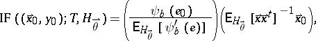
where $r _ { i } = y _ { i } - \overset{\rightharpoonup} { x } _ { i } ^ { t } T _ { n }$ are the residuals. If the Huber function $\psi_b$ is used, the influence function of $T$ at $H _ { \overset{\rightharpoonup}{ \theta } }$ equals
 | (a2) |
where $e _ { 0 } = y _ { 0 } - \overset{\rightharpoonup} { x } _ { 0 } ^ { t} \overset{\rightharpoonup} { \theta }$. The first factor of (a2) is the influence of the vertical error $e_0$. It is bounded, which makes this estimator more robust than least squares (cf. also Least squares, method of). The second factor is the influence of the position $\overset{\rightharpoonup} { x }_{0}$. Unfortunately, this factor is unbounded, hence a single outlying $\overset{\rightharpoonup} { x } _ { j }$ (i.e., a horizontal outlier) will almost completely determine the fit, as shown in [a2]. Therefore the breakdown value $\varepsilon ^ { * } ( T ) = 0$.
To obtain a bounded influence function, generalized M-estimators [a2] are defined by
\begin{equation*} \sum _ { i = 1 } ^ { n } \eta ( \overset{\rightharpoonup} { x } _ { i } , r _ { i } ) \overset{\rightharpoonup}{ x } _ { i } = \overset{\rightharpoonup}{ 0 }, \end{equation*}
for some real function $ \eta $. The influence function of $T$ at $H _ { \overset{\rightharpoonup}{ \theta } }$ now becomes
\begin{equation} \tag{a3} \operatorname { IF } ( ( \overset{\rightharpoonup} { x } _ { 0 } , y _ { 0 } ) ; T , H _ { \overset{\rightharpoonup}{ \theta } } ) = \eta ( \overset{\rightharpoonup} { x } _ { 0 } , e _ { 0 } ) M ^ { - 1 } \overset{\rightharpoonup} { x } _ { 0 }, \end{equation}
where $e _ { 0 } = y _ { 0 } - \overset{\rightharpoonup} { x } _ { 0 } ^ { t} \overset{\rightharpoonup} { \theta }$ and $M = \int ( \partial / \partial e ) \eta ( \overset{\rightharpoonup} { x } , e ) \overset{\rightharpoonup} { x } \overset{\rightharpoonup} {x } ^ { t } d H _ { \overset{\rightharpoonup} { \theta } } ( \overset{\rightharpoonup} { x } , y )$. For an appropriate choice of the function $ \eta $, the influence function (a3) is bounded, but still the breakdown value $\varepsilon ^ { * } ( T )$ goes down to zero when the number of parameters $p$ increases.
To repair this, P.J. Rousseeuw and V.J. Yohai [a5] have introduced S-estimators. An S-estimator $T _ { n }$ minimizes $s ( r _ { 1 } , \dots , r _ { n } )$, where $r _ { i } = y _ { i } - \overset{\rightharpoonup} { x } _ { i } ^ { t } T _ { n }$ are the residuals and $s ( r _ { 1 } , \dots , r _ { n } )$ is the robust scale estimator defined as the solution of
\begin{equation*} \frac { 1 } { n } \sum _ { i = 1 } ^ { n } \rho \left( \frac { r_i } { s } \right) = K, \end{equation*}
where $K$ is taken to be $\int \rho ( u ) d \Phi ( u )$. The function $\rho$ must satisfy $\rho ( - u ) = \rho ( u )$ and $\rho ( 0 ) = 0$ and be continuously differentiable, and there must be a constant $c > 0$ such that $\rho$ is strictly increasing on $[ 0 , c ]$ and constant on $[ c , \infty )$. Any S-estimator has breakdown value $\varepsilon ^ { * } ( T ) = 1 / 2$ in all dimensions, and it is asymptotically normal with the same asymptotic covariance as the M-estimator with that function $\rho$. The S-estimators have also been generalized to multivariate location and scatter matrices, in [a6], and they enjoy the same properties.
References
| [a1] | P.J. Huber, "Robust estimation of a location parameter" Ann. Math. Stat. , 35 (1964) pp. 73–101 |
| [a2] | F.R. Hampel, E.M. Ronchetti, P.J. Rousseeuw, W.A. Stahel, "Robust statistics: The approach based on influence functions" , Wiley (1986) |
| [a3] | P.J. Huber, "Robust statistics" , Wiley (1981) |
| [a4] | R.A. Maronna, "Robust M-estimators of multivariate location and scatter" Ann. Statist. , 4 (1976) pp. 51–67 |
| [a5] | P.J. Rousseeuw, V.J. Yohai, "Robust regression by means of S-estimators" J. Franke (ed.) W. Härdle (ed.) R.D. Martin (ed.) , Robust and Nonlinear Time Ser. Analysis , Lecture Notes Statistics , 26 , Springer (1984) pp. 256–272 |
| [a6] | P.J. Rousseeuw, A. Leroy, "Robust regression and outlier detection" , Wiley (1987) |
M-estimator. Encyclopedia of Mathematics. URL: http://encyclopediaofmath.org/index.php?title=M-estimator&oldid=12651