Interpolation formula
A formula for the approximate calculation of values of a function  by replacing it by a function
 |
that is simple in a certain sense and belongs to a certain class. The parameters  ,
,  , are chosen in such a way that the values of
  coincide with the known values of
  on a given set of
  distinct values of the argument:
 | (1) |
This method of approximately representing a function is called interpolation, and the points  at which (1) should hold are called interpolation nodes. Instead of the simplest condition (1), the values of some quantity related to
  may also be given, e.g. the values of a derivative of
  at interpolation nodes.
The method of linear interpolation is the most widespread among the interpolation methods. The approximation is now looked for in the class of (generalized) polynomials
 | (2) |
in some fixed system of functions  . In order for the interpolation polynomial (2) to exist for any function
  defined on an interval
  , and for any choice of
  nodes
nodes  ,
,  if
if  , it is necessary and sufficient that
  is a Chebyshev system of functions on
  . The interpolation polynomial will, moreover, be unique and its coefficients
  can be found by directly solving (1).
For  one often takes: the sequences of powers of
  ,
,
 |
the sequence of trigonometric functions,
 |
or the sequence of exponential functions,
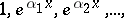 |
where  is a sequence of distinct real numbers.
When interpolating by algebraic polynomials
 | (3) |
the system  is
is
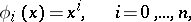 | (4) |
while (1) has the form
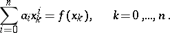 | (5) |
The system (4) is a Chebyshev system, which ensures the existence and uniqueness of the interpolation polynomial (3). A property of (4) is the possibility of obtaining an explicit representation of the interpolation polynomial (3) without immediately having to solve (5). One of the explicit forms of (3),
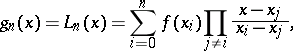 | (6) |
is called the Lagrange interpolation polynomial (cf. Lagrange interpolation formula). If the derivative  is continuous, the remainder of (6) can be written as
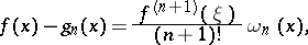 | (7) |
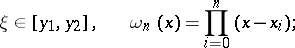 |
where  ;
;  . The value of the remainder (7) depends, in particular, on the values of
  . The choice of interpolation nodes for which
  is minimal, is of interest. The distribution of the nodes is optimal in this sense if the roots
 |
of the polynomial
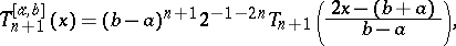 |
which deviates least from zero on  , are taken as the nodes. Here
  is the Chebyshev polynomial of degree
  (cf. Chebyshev polynomials).
There is a number of other explicit representations of (3) that are more useful for solving this or another practical interpolation problem (cf., e.g., Bessel interpolation formula; Gauss interpolation formula; Newton interpolation formula; Stirling interpolation formula; Steffensen interpolation formula; Everett interpolation formula). If it is difficult to estimate in advance the degree of the interpolation polynomial that is necessary for attaining the error desired (e.g., when interpolating a table), then one takes recourse to the Aitken scheme. In this scheme interpolation polynomials of increasing degrees are constructed sequentially, thus making it possible to control the accuracy in the computational process. Another approach to the construction of interpolation formulas can be found in Fraser diagram.
The Hermite interpolation formula gives the solution to the problem of the algebraic interpolation of the values of a function and its derivatives at interpolation nodes.
References
| [1] | I.S. Berezin, N.P. Zhidkov, "Computing methods" , Pergamon (1973) (Translated from Russian) |
| [2] | N.S. Bakhvalov, "Numerical methods: analysis, algebra, ordinary differential equations" , MIR (1977) (Translated from Russian) |
Comments
Many interpolation formulas are contained in [a1]–[a3].
Consider the interpolation problem of finding a polynomial  of degree
  satisfying the conditions
 | (a1) |
where the  are
are  distinct knots, and there are precisely
  equations in (a1). If for each
  the orders of the derivatives occurring in (a1) form an unbroken series
  , one has Hermite interpolation. (In case
  for all
  , i.e. if no interpolation conditions involving derivatives occur in (a1), one has Lagrange interpolation.) If gaps (lacunae) occur, one speaks of lacunary interpolation or Birkhoff interpolation. The pairs
  which occur in (a1) are conveniently described in terms of an interpolation matrix
  of size
  ,
,  ,
,  ,
,  , where
  if
if  does occur in (a1) and
  otherwise. The matrix
  is called regular if (a1) is solvable for all choices of the
  and
and  and singular otherwise.
More generally, let  be a system of linearly independent
  -times continuously-differentiable real-valued functions on an interval
  or on the circle. Instead of polynomials now consider linear combinations
  . A matrix of zeros and ones
  ,
,  ,
,  , is an interpolation matrix if there are precisely
  ones in
  (and, usually, if there are no rows of zeros in
  ; this means that all knots do occur at least once in an interpolation condition). Let
  be a set of knots, i.e.
  distinct points of the interval or circle. Finally, for each
  such that
  let there be given a number
  . These data
  define a Birkhoff interpolation problem:
 | (a2) |
 |
The pair  is called regular if (a2) is solvable for all choices of the
  .
.
For each  such that
  , consider the row vector of length
  ,
,
 |
For varying  such that
  one thus finds
  row vectors which together make up an
  matrix. The pair
  is regular if and only if this matrix is invertible. Its determinant, where the pairs
  with
with  are ordered lexicographically, is denoted
  .
.
Suppose that the  are the values
  of the derivatives of some function
  at the knots. Then a simple formula for the solution of the interpolation problem (a2) follows from Cramer's rule. Indeed, if
  denotes the determinant obtained by replacing
  with
with  in the formula for
  , then
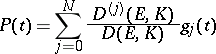 | (a3) |
See also Hermite interpolation formula.
References
| [a1] | P.J. Davis, "Interpolation and approximation" , Dover, reprint (1975) pp. 108–126 |
| [a2] | F.B. Hildebrand, "Introduction to numerical analysis" , McGraw-Hill (1974) |
| [a3] | J.F. Steffenson, "Interpolation" , Chelsea, reprint (1950) |
| [a4] | G.G. Lorentz, K. Jetter, S.D. Riemenschneider, "Birkhoff interpolation" , Addison-Wesley (1983) |
Interpolation formula. Encyclopedia of Mathematics. URL: http://encyclopediaofmath.org/index.php?title=Interpolation_formula&oldid=14575