Difference between revisions of "Dempster-Shafer theory"
Ulf Rehmann (talk | contribs) m (moved Dempster–Shafer theory to Dempster-Shafer theory: ascii title) |
m (AUTOMATIC EDIT (latexlist): Replaced 124 formulas out of 137 by TEX code with an average confidence of 2.0 and a minimal confidence of 2.0.) |
||
| Line 1: | Line 1: | ||
| + | <!--This article has been texified automatically. Since there was no Nroff source code for this article, | ||
| + | the semi-automatic procedure described at https://encyclopediaofmath.org/wiki/User:Maximilian_Janisch/latexlist | ||
| + | was used. | ||
| + | If the TeX and formula formatting is correct, please remove this message and the {{TEX|semi-auto}} category. | ||
| + | |||
| + | Out of 137 formulas, 124 were replaced by TEX code.--> | ||
| + | |||
| + | {{TEX|semi-auto}}{{TEX|partial}} | ||
''mathematical theory of evidence, belief function theory'' | ''mathematical theory of evidence, belief function theory'' | ||
| Line 6: | Line 14: | ||
==Axiomatic approach.== | ==Axiomatic approach.== | ||
| − | Let | + | Let $\Xi$ be a finite set of elements, called elementary events. Any subset of $\Xi$ with cardinality $1$ is also called a frame of discernment and any other subset of $\Xi$ is called a composite event. |
| − | The central concept of a belief function is understood as any function | + | The central concept of a belief function is understood as any function $\operatorname{Bel}: 2 ^ { \Xi } \rightarrow [ 0,1 ]$ fulfilling the axioms: |
| − | + | $\operatorname { Bel } ( \emptyset ) = 0$; | |
| − | + | $\operatorname { Bel } ( \Xi ) = 1$; | |
| − | + | $\operatorname { Bel } ( A _ { 1 } \cup \ldots \cup A _ { k } ) \geq$ | |
| − | + | \begin{equation*} \geq \sum _ { I \subseteq \{ 1 , \ldots , k \} , I \neq \emptyset } ( - 1 ) ^ { | I | + 1 } \operatorname { Bel } ( \bigcap _ { i \in I } A _ { i } ). \end{equation*} | |
| − | Due to the last axiom, a belief function | + | Due to the last axiom, a belief function $\operatorname { Bel}$ is actually a Choquet capacity, monotone of infinite order (cf. also [[Capacity|Capacity]]). By introducing the so-called basic probability assignment function (bpa function), or mass function, $m : 2 ^ { \Xi } \rightarrow [ 0,1 ]$ such that $\sum _ { A \in 2 ^ \Xi } m ( A ) = 1$ and $m ( \emptyset ) = 0$, then $\operatorname { Bel}$ can be expressed as $\operatorname { Bel } ( A ) = \sum _ { B \subseteq A } m ( B )$. Other uncertainty measures can also be defined, like the plausibility function $\operatorname { Pl } ( A ) = 1 - \operatorname { Bel } ( \Xi - A )$ and the commonality function $Q ( A ) = \sum _ { B ; A \subseteq B} m ( B ) $. Given one of these functions $\operatorname { Bel}$, $\text{Pl}$, $m$, $Q$, any other of them may be deterministically derived. Hence the function $m$ is frequently used in the definition of further concepts, e.g., any set $A$ with $m ( A ) > 0$ is called a focal point of the belief function. If $m ( \Xi ) = 1$, then the belief function is called vacuous. |
| − | Another central concept, the rule of combination of two independent belief functions | + | Another central concept, the rule of combination of two independent belief functions $\operatorname{Bel}_{E _ { 1 }}$, $\operatorname{Bel}_{E _ { 2 }}$ over the same frame of discernment (the so-called Dempster rule of evidence combination), denoted by $\operatorname{Bel} _ { E _ { 1 } , E _ { 2 } } = \operatorname{Bel} _ { E _ { 1 } } \oplus \operatorname{Bel} _ { E _ { 2 } }$, is defined as follows: |
| − | + | \begin{equation*} m _ { E _ { 1 } , E _ { 2 } } ( A ) = c . \sum _ { B , C ; A = B \bigcap C } m _ { E _ { 1 } } ( B ) .m _ { E _ { 2 } } ( C ) \end{equation*} | |
| − | (with | + | (with $c$ a constant normalizing the sum of $m _ { E _{1} , E _ { 2 }}$ to $1$). |
| − | Suppose that a frame of discernment | + | Suppose that a frame of discernment $\Xi$ is equal to the cross product of domains $\Xi _ { 1 } , \dots , \Xi _ { n }$, with $n$ discrete variables $X _ { 1 } , \ldots , X _ { n }$ spanning the space $\Xi$. Let $( x _ { 1 } , \dots , x _ { n } )$ be a vector in the space spanned by the variables $X _ { 1 } , \dots , X _ { n }$. Its projection onto the subspace spanned by the variables $X _ { j _ { 1 } } , \dots , X _ { j _ { k } }$ (with $j_1 , \dots , j _ { k }$ distinct indices from $1 , \dots , n$) is then the vector $( x _ { j _ { 1 } } , \dots , x _ { j _ { k } } )$. The vector $( x _ { 1 } , \dots , x _ { n } )$ is also called an extension of $( x _ { j _ { 1 } } , \dots , x _ { j _ { k } } )$. The projection of a set $A$ of such vectors is the set <img align="absmiddle" border="0" src="https://www.encyclopediaofmath.org/legacyimages/d/d130/d130060/d13006047.png"/> of projections of all individual vectors from $A$ onto $X _ { j _ { 1 } } , \dots , X _ { j _ { k } }$. $A$ is also called an extension of <img align="absmiddle" border="0" src="https://www.encyclopediaofmath.org/legacyimages/d/d130/d130060/d13006051.png"/>. $A$ is called a vacuous extension of <img align="absmiddle" border="0" src="https://www.encyclopediaofmath.org/legacyimages/d/d130/d130060/d13006053.png"/> if (and only if) $A$ contains all possible extensions of each individual vector in <img align="absmiddle" border="0" src="https://www.encyclopediaofmath.org/legacyimages/d/d130/d130060/d13006055.png"/>. The fact that $A$ is a vacuous extension of $B$ onto $X _ { 1 } , \ldots , X _ { n }$ is denoted by $A = B ^ { \uparrow X _ { 1 } , \ldots , X _ { n } }$. |
| − | Let | + | Let $m$ be a basic probability assignment function on the space of discernment spanned by the set of variables $X = \{ X _ { 1 } , \dots , X _ { n } \}$, and let $\operatorname { Bel}$ be the corresponding belief function. Let $Y$ be a subset of $X$. The projection operator (or marginalization operator) $\downarrow$ of $\operatorname { Bel}$ (or $m$) onto the subspace spanned by $Y$ is defined as |
| − | + | \begin{equation*} m ^ { \downarrow Y } ( B ) = \sum _ { A : B = A ^ { \downarrow Y } } m ( A ). \end{equation*} | |
| − | The vacuous extension operator | + | The vacuous extension operator $\uparrow$ of $\operatorname { Bel}$ (or $m$) from $Y$ onto the superspace spanned by $X$ is defined as follows: for any $A$ in $X$ and any $B$ in $Y$ such that $A = B ^ { \uparrow X }$ one has $m ^ { \uparrow X } ( A ) = m ( B )$, and for any other $A$ from $X$, $m ^ { \uparrow X } ( A ) = 0$. To denote that a belief function $\operatorname { Bel}$ is defined over the space spanned by the set of variables $X$ one frequently writes $\operatorname{Bel}_X$. By convention, if one wants to combine, using Dempster's rule, two belief functions not sharing the frame of discernment, then one looks for the closest common vacuous extension of their frames of discernment without explicitly mentioning this. |
| − | The last important concept of Dempster–Shafer theory is the Dempster rule of conditioning: Let | + | The last important concept of Dempster–Shafer theory is the Dempster rule of conditioning: Let $B$ be a subset of $\Xi$, called evidence, and let $m _{B}$ be a basic probability assignment such that $m _ { B } ( B ) = 1$ and $m _ { B } ( A ) = 0$ for all $A$ different from $B$. Then the conditional belief function $\operatorname {Bel} ( \cdot | | B )$, representing the belief function $\operatorname { Bel}$ conditioned on evidence $B$, is defined as: |
| − | + | \begin{equation*} \operatorname{Bel} ( \cdot | | B ) =\operatorname{Bel} \bigoplus \operatorname{Bel}_B . \end{equation*} | |
| − | The conditioning as defined by the above rule is the foundation of reasoning in Dempster–Shafer theory: One starts with a belief function <img align="absmiddle" border="0" src="https://www.encyclopediaofmath.org/legacyimages/d/d130/d130060/d13006098.png" /> defined in a multi-variable space | + | The conditioning as defined by the above rule is the foundation of reasoning in Dempster–Shafer theory: One starts with a belief function <img align="absmiddle" border="0" src="https://www.encyclopediaofmath.org/legacyimages/d/d130/d130060/d13006098.png"/> defined in a multi-variable space $X$ (being one's knowledge), makes certain observations on the values taken by some observational variables $Y \subset X$, e.g. $Y _ { 1 } \in \{ y _ { 1 , 1} , y _ { 1 , 3} , y _ { 1 ,8} \}$, denotes this knowledge by $m _{Y _ { 1 } , \operatorname{obs}} ( \{ y _ { 1,1 } , y _ { 1,3 } , y _ { 1,8 } \} ) = 1$, and then one wishes to know what value will be taken by a predicted variable $Z \in X$. To that end one calculates the belief for the predicted variable as |
| − | <table class="eq" style="width:100%;"> <tr><td | + | <table class="eq" style="width:100%;"> <tr><td style="width:94%;text-align:center;" valign="top"><img align="absmiddle" border="0" src="https://www.encyclopediaofmath.org/legacyimages/d/d130/d130060/d130060104.png"/></td> </tr></table> |
| − | Due to the large space, the calculation of such a margin is prohibitive unless one can decompose <img align="absmiddle" border="0" src="https://www.encyclopediaofmath.org/legacyimages/d/d130/d130060/d130060105.png" /> into a set of "smaller" belief functions <img align="absmiddle" border="0" src="https://www.encyclopediaofmath.org/legacyimages/d/d130/d130060/d130060106.png" /> over a set | + | Due to the large space, the calculation of such a margin is prohibitive unless one can decompose <img align="absmiddle" border="0" src="https://www.encyclopediaofmath.org/legacyimages/d/d130/d130060/d130060105.png"/> into a set of "smaller" belief functions <img align="absmiddle" border="0" src="https://www.encyclopediaofmath.org/legacyimages/d/d130/d130060/d130060106.png"/> over a set $H$ of subsets of $X$ such that |
| − | + | \begin{equation*} \operatorname{Bel}_{X,\text{known}}= \bigoplus _ { h_ { i } \in H } \operatorname{Bel} _ { h_i, \text{know} }. \end{equation*} | |
| − | The set | + | The set $H$ is hence a [[Hypergraph|hypergraph]]. If $H$ is a hypertree (a special type of hypergraph), then one can efficiently reason using the Shenoy–Shafer algorithms [[#References|[a7]]]. Any hypergraph can be transformed into a hypertree, but the task aiming to obtain the best hypertree for reasoning (with smallest subsets in $H$) is prohibitive ($\cal N P$-hard, cf. also [[NP|$\cal N P$]]), hence suboptimal solutions are elaborated. In the Shenoy–Shafer framework, both forward, backward and mixed reasoning is possible. |
| − | Note that in the above decomposition it is not assumed that the <img align="absmiddle" border="0" src="https://www.encyclopediaofmath.org/legacyimages/d/d130/d130060/d130060116.png" /> can be calculated in any way from <img align="absmiddle" border="0" src="https://www.encyclopediaofmath.org/legacyimages/d/d130/d130060/d130060117.png" />. As | + | Note that in the above decomposition it is not assumed that the <img align="absmiddle" border="0" src="https://www.encyclopediaofmath.org/legacyimages/d/d130/d130060/d130060116.png"/> can be calculated in any way from <img align="absmiddle" border="0" src="https://www.encyclopediaofmath.org/legacyimages/d/d130/d130060/d130060117.png"/>. As $\operatorname { Bel}$ is known to have so-called graphoidal properties [[#References|[a8]]], a decomposition similar to Bayesian networks for probability distributions has also been studied. An a priori-condition belief function $\operatorname {Bel} _ { Z | Y}$ of variables $Z$ given $Y$ (defined over $Z \cup Y$), both sets with empty intersection and both subsets of $X$, is introduced as: |
| − | + | \begin{equation*} \operatorname { Bel } _ { X } ^ { \downarrow Z \bigcup Y } = \operatorname { Bel } _ { Z | Y } \bigoplus \operatorname { Bel } _ { X } ^ { \downarrow Y }. \end{equation*} | |
| − | In general, many such functions may exist. In these settings one says that for a belief function | + | In general, many such functions may exist. In these settings one says that for a belief function $\operatorname{Bel}_X$ two non-intersecting sets of variables $T \subseteq X$ and $R \subseteq X$ are independent given $X - T - R$ if |
| − | + | \begin{equation*} \operatorname { Bel } _ { X } = \operatorname { Bel } ^ { \downarrow X - R _ { T | X - T - R} } \bigoplus \operatorname { Bel } ^ { \downarrow X - T _ { R | X - T - R} } \bigoplus \operatorname { Bel } ^ { \downarrow X - T - R _ { X } }. \end{equation*} | |
| − | The a priori-conditional belief function is usually not a belief function, as it usually does not match the third axiom for belief functions, and even may take negative values (and so do the corresponding plausibility and mass functions). Only conditional commonality functions are always non-negative everywhere. As a partial remedy, the so-called | + | The a priori-conditional belief function is usually not a belief function, as it usually does not match the third axiom for belief functions, and even may take negative values (and so do the corresponding plausibility and mass functions). Only conditional commonality functions are always non-negative everywhere. As a partial remedy, the so-called $K$ function has been proposed: |
| − | <table class="eq" style="width:100%;"> <tr><td | + | <table class="eq" style="width:100%;"> <tr><td style="width:94%;text-align:center;" valign="top"><img align="absmiddle" border="0" src="https://www.encyclopediaofmath.org/legacyimages/d/d130/d130060/d130060132.png"/></td> </tr></table> |
| − | It may be viewed as an analogue of the true mass function for "a priori conditionals" , as it is non-negative and for any fixed value of | + | It may be viewed as an analogue of the true mass function for "a priori conditionals" , as it is non-negative and for any fixed value of $Y$ the sum over $Z$ equals $1$. Contrary to intuitions with probability distributions, the combination of an a priori conditional belief function with a (true) belief function by Dempster's rule need not lead to a belief function. Hence such a priori functions are poorly investigated so far (2000). |
==Naive case-based approach.== | ==Naive case-based approach.== | ||
| Line 75: | Line 83: | ||
==Subjectivist approach.== | ==Subjectivist approach.== | ||
| − | One assumes that among the elements of the set | + | One assumes that among the elements of the set $\Omega$, called "worlds" , one world corresponds to the "actual world" . There is an agent who does not know which world is the actual world and who can only express the strength of his/her opinion (called the degree of belief) that the actual world belongs to a certain subset of $\Omega$. One such approach is the so-called transferable belief model [[#References|[a10]]]. Besides the two already mentioned rules of Dempster (combination and conditioning), many more rules handling various sources of evidence have been added, including disjunctive rules of combination, alpha-junctions rules, cautious rules, pignistic transformation, a specialization concept, a measure of information content, canonical decomposition, concepts of confidence and diffidence, and a generalized Bayesian theorem. Predominantly, the qualitative behaviour of subjectively assigned beliefs is studied. So far (as of 2000), no attempt paralleling the subjective probability approach of B. de Finetti has been made to bridge the gap between subjective belief assignment and observed frequencies. |
====References==== | ====References==== | ||
| − | <table>< | + | <table><tr><td valign="top">[a1]</td> <td valign="top"> J. Cano, M. Delgado, S. Moral, "An axiomatic framework for propagating uncertainty in directed acyclic networks" ''Internat. J. Approximate Reasoning'' , '''8''' (1993) pp. 253–280</td></tr><tr><td valign="top">[a2]</td> <td valign="top"> A.P. Dempster, "Upper and lower probabilities induced by a multi-valued mapping" ''Ann. Math. Stat.'' , '''38''' (1967) pp. 325–339</td></tr><tr><td valign="top">[a3]</td> <td valign="top"> M.A. Kłopotek, S.T. Wierzchoń, "On marginally correct approximations of Dempster–Shafer belief functions from data" , ''Proc. IPMU'96 (Information Processing and Management of Uncertainty), Grenada (Spain), 1-5 July'' , '''II''' , Univ. Granada (1996) pp. 769–774</td></tr><tr><td valign="top">[a4]</td> <td valign="top"> M.A. Kłopotek, S.T. Wierzchoń, "Qualitative versus quantitative interpretation of the mathematical theory of evidence" Z.W.Raś (ed.) A. Skowron (ed.) , ''Foundations of Intelligent Systems 7. Proc. ISMIS'97 (Charlotte NC, 15-17 Oct., 1997)'' , ''Lecture Notes in Artificial Intelligence'' , '''1325''' , Springer (1997) pp. 391–400</td></tr><tr><td valign="top">[a5]</td> <td valign="top"> M.A. Kłopotek, "On (anti)conditional independence in Dempster–Shafer theory" ''J. Mathware and Softcomputing'' , '''5''' : 1 (1998) pp. 69–89</td></tr><tr><td valign="top">[a6]</td> <td valign="top"> G. Shafer, "A mathematical theory of evidence" , Princeton Univ. Press (1976)</td></tr><tr><td valign="top">[a7]</td> <td valign="top"> P. Shenoy, G. Shafer, "Axioms for probability and belief-function propagation" R.D. Shachter (ed.) T.S. Levitt (ed.) L.N. Kanal (ed.) J.F. Lemmer (ed.) , ''Uncertainty in Artificial Intelligence'' , '''4''' , Elsevier (1990)</td></tr><tr><td valign="top">[a8]</td> <td valign="top"> P.P. Shenoy, "Conditional independence in valuation based systems" ''Internat. J. Approximate Reasoning'' , '''109''' (1994)</td></tr><tr><td valign="top">[a9]</td> <td valign="top"> A. Skowron, J.W. Grzymała-Busse, "From rough set theory to evidence theory" R.R. Yager (ed.) J. Kasprzyk (ed.) M. Fedrizzi (ed.) , ''Advances in the Dempster–Shafer Theory of Evidence'' , Wiley (1994) pp. 193–236</td></tr><tr><td valign="top">[a10]</td> <td valign="top"> Ph. Smets, "Numerical representation of uncertainty" D.M. Gabbay (ed.) Ph. Smets (ed.) , ''Handbook of Defeasible Reasoning and Uncertainty Management Systems'' , '''3''' , Kluwer Acad. Publ. (1998) pp. 265–309</td></tr><tr><td valign="top">[a11]</td> <td valign="top"> S.T. Wierzchoń, M.A. Kłopotek, "Modified component valuations in valuation based systems as a way to optimize query processing" ''J. Intelligent Information Syst.'' , '''9''' (1997) pp. 157–180</td></tr></table> |
Revision as of 16:58, 1 July 2020
mathematical theory of evidence, belief function theory
A theory initiated by A.P. Dempster [a2] and later developed by G. Shafer [a6]. It deals with the representation of non-probabilistic uncertainty about sets of facts (belief function) and the accumulation of "evidence" stemming from independent sources (Dempster's rule of evidence combination) and with reasoning under incomplete information (Dempster's rule of conditioning); see below. Extensions to infinite countable sets and continuous sets have been studied. However, below finite sets of facts (elementary events) are considered.
As with probability theory, four different approaches to handling Dempster–Shafer theory may be distinguished: the axiomatic approach (formal properties of belief functions are analyzed); the naive case-based approach (a direct case-based interpretation of properties of belief functions is sought); the in-the-limit approach (properties of the belief function are considered as in-the-limit properties of sets of cases); and the subjectivist approach (predominantly, the qualitative behaviour of subjectively assigned beliefs is studied, no case-based interpretation is sought and belief is considered as a subjective basis for decision-making).
Axiomatic approach.
Let $\Xi$ be a finite set of elements, called elementary events. Any subset of $\Xi$ with cardinality $1$ is also called a frame of discernment and any other subset of $\Xi$ is called a composite event.
The central concept of a belief function is understood as any function $\operatorname{Bel}: 2 ^ { \Xi } \rightarrow [ 0,1 ]$ fulfilling the axioms:
$\operatorname { Bel } ( \emptyset ) = 0$;
$\operatorname { Bel } ( \Xi ) = 1$;
$\operatorname { Bel } ( A _ { 1 } \cup \ldots \cup A _ { k } ) \geq$
\begin{equation*} \geq \sum _ { I \subseteq \{ 1 , \ldots , k \} , I \neq \emptyset } ( - 1 ) ^ { | I | + 1 } \operatorname { Bel } ( \bigcap _ { i \in I } A _ { i } ). \end{equation*}
Due to the last axiom, a belief function $\operatorname { Bel}$ is actually a Choquet capacity, monotone of infinite order (cf. also Capacity). By introducing the so-called basic probability assignment function (bpa function), or mass function, $m : 2 ^ { \Xi } \rightarrow [ 0,1 ]$ such that $\sum _ { A \in 2 ^ \Xi } m ( A ) = 1$ and $m ( \emptyset ) = 0$, then $\operatorname { Bel}$ can be expressed as $\operatorname { Bel } ( A ) = \sum _ { B \subseteq A } m ( B )$. Other uncertainty measures can also be defined, like the plausibility function $\operatorname { Pl } ( A ) = 1 - \operatorname { Bel } ( \Xi - A )$ and the commonality function $Q ( A ) = \sum _ { B ; A \subseteq B} m ( B ) $. Given one of these functions $\operatorname { Bel}$, $\text{Pl}$, $m$, $Q$, any other of them may be deterministically derived. Hence the function $m$ is frequently used in the definition of further concepts, e.g., any set $A$ with $m ( A ) > 0$ is called a focal point of the belief function. If $m ( \Xi ) = 1$, then the belief function is called vacuous.
Another central concept, the rule of combination of two independent belief functions $\operatorname{Bel}_{E _ { 1 }}$, $\operatorname{Bel}_{E _ { 2 }}$ over the same frame of discernment (the so-called Dempster rule of evidence combination), denoted by $\operatorname{Bel} _ { E _ { 1 } , E _ { 2 } } = \operatorname{Bel} _ { E _ { 1 } } \oplus \operatorname{Bel} _ { E _ { 2 } }$, is defined as follows:
\begin{equation*} m _ { E _ { 1 } , E _ { 2 } } ( A ) = c . \sum _ { B , C ; A = B \bigcap C } m _ { E _ { 1 } } ( B ) .m _ { E _ { 2 } } ( C ) \end{equation*}
(with $c$ a constant normalizing the sum of $m _ { E _{1} , E _ { 2 }}$ to $1$).
Suppose that a frame of discernment $\Xi$ is equal to the cross product of domains $\Xi _ { 1 } , \dots , \Xi _ { n }$, with $n$ discrete variables $X _ { 1 } , \ldots , X _ { n }$ spanning the space $\Xi$. Let $( x _ { 1 } , \dots , x _ { n } )$ be a vector in the space spanned by the variables $X _ { 1 } , \dots , X _ { n }$. Its projection onto the subspace spanned by the variables $X _ { j _ { 1 } } , \dots , X _ { j _ { k } }$ (with $j_1 , \dots , j _ { k }$ distinct indices from $1 , \dots , n$) is then the vector $( x _ { j _ { 1 } } , \dots , x _ { j _ { k } } )$. The vector $( x _ { 1 } , \dots , x _ { n } )$ is also called an extension of $( x _ { j _ { 1 } } , \dots , x _ { j _ { k } } )$. The projection of a set $A$ of such vectors is the set  of projections of all individual vectors from $A$ onto $X _ { j _ { 1 } } , \dots , X _ { j _ { k } }$. $A$ is also called an extension of
  . $A$ is called a vacuous extension of
  if (and only if) $A$ contains all possible extensions of each individual vector in
  . The fact that $A$ is a vacuous extension of $B$ onto $X _ { 1 } , \ldots , X _ { n }$ is denoted by $A = B ^ { \uparrow X _ { 1 } , \ldots , X _ { n } }$.
Let $m$ be a basic probability assignment function on the space of discernment spanned by the set of variables $X = \{ X _ { 1 } , \dots , X _ { n } \}$, and let $\operatorname { Bel}$ be the corresponding belief function. Let $Y$ be a subset of $X$. The projection operator (or marginalization operator) $\downarrow$ of $\operatorname { Bel}$ (or $m$) onto the subspace spanned by $Y$ is defined as
\begin{equation*} m ^ { \downarrow Y } ( B ) = \sum _ { A : B = A ^ { \downarrow Y } } m ( A ). \end{equation*}
The vacuous extension operator $\uparrow$ of $\operatorname { Bel}$ (or $m$) from $Y$ onto the superspace spanned by $X$ is defined as follows: for any $A$ in $X$ and any $B$ in $Y$ such that $A = B ^ { \uparrow X }$ one has $m ^ { \uparrow X } ( A ) = m ( B )$, and for any other $A$ from $X$, $m ^ { \uparrow X } ( A ) = 0$. To denote that a belief function $\operatorname { Bel}$ is defined over the space spanned by the set of variables $X$ one frequently writes $\operatorname{Bel}_X$. By convention, if one wants to combine, using Dempster's rule, two belief functions not sharing the frame of discernment, then one looks for the closest common vacuous extension of their frames of discernment without explicitly mentioning this.
The last important concept of Dempster–Shafer theory is the Dempster rule of conditioning: Let $B$ be a subset of $\Xi$, called evidence, and let $m _{B}$ be a basic probability assignment such that $m _ { B } ( B ) = 1$ and $m _ { B } ( A ) = 0$ for all $A$ different from $B$. Then the conditional belief function $\operatorname {Bel} ( \cdot | | B )$, representing the belief function $\operatorname { Bel}$ conditioned on evidence $B$, is defined as:
\begin{equation*} \operatorname{Bel} ( \cdot | | B ) =\operatorname{Bel} \bigoplus \operatorname{Bel}_B . \end{equation*}
The conditioning as defined by the above rule is the foundation of reasoning in Dempster–Shafer theory: One starts with a belief function  defined in a multi-variable space $X$ (being one's knowledge), makes certain observations on the values taken by some observational variables $Y \subset X$, e.g. $Y _ { 1 } \in \{ y _ { 1 , 1} , y _ { 1 , 3} , y _ { 1 ,8} \}$, denotes this knowledge by $m _{Y _ { 1 } , \operatorname{obs}} ( \{ y _ { 1,1 } , y _ { 1,3 } , y _ { 1,8 } \} ) = 1$, and then one wishes to know what value will be taken by a predicted variable $Z \in X$. To that end one calculates the belief for the predicted variable as
 |
Due to the large space, the calculation of such a margin is prohibitive unless one can decompose  into a set of "smaller" belief functions
  over a set $H$ of subsets of $X$ such that
\begin{equation*} \operatorname{Bel}_{X,\text{known}}= \bigoplus _ { h_ { i } \in H } \operatorname{Bel} _ { h_i, \text{know} }. \end{equation*}
The set $H$ is hence a hypergraph. If $H$ is a hypertree (a special type of hypergraph), then one can efficiently reason using the Shenoy–Shafer algorithms [a7]. Any hypergraph can be transformed into a hypertree, but the task aiming to obtain the best hypertree for reasoning (with smallest subsets in $H$) is prohibitive ($\cal N P$-hard, cf. also $\cal N P$), hence suboptimal solutions are elaborated. In the Shenoy–Shafer framework, both forward, backward and mixed reasoning is possible.
Note that in the above decomposition it is not assumed that the  can be calculated in any way from
  . As $\operatorname { Bel}$ is known to have so-called graphoidal properties [a8], a decomposition similar to Bayesian networks for probability distributions has also been studied. An a priori-condition belief function $\operatorname {Bel} _ { Z | Y}$ of variables $Z$ given $Y$ (defined over $Z \cup Y$), both sets with empty intersection and both subsets of $X$, is introduced as:
\begin{equation*} \operatorname { Bel } _ { X } ^ { \downarrow Z \bigcup Y } = \operatorname { Bel } _ { Z | Y } \bigoplus \operatorname { Bel } _ { X } ^ { \downarrow Y }. \end{equation*}
In general, many such functions may exist. In these settings one says that for a belief function $\operatorname{Bel}_X$ two non-intersecting sets of variables $T \subseteq X$ and $R \subseteq X$ are independent given $X - T - R$ if
\begin{equation*} \operatorname { Bel } _ { X } = \operatorname { Bel } ^ { \downarrow X - R _ { T | X - T - R} } \bigoplus \operatorname { Bel } ^ { \downarrow X - T _ { R | X - T - R} } \bigoplus \operatorname { Bel } ^ { \downarrow X - T - R _ { X } }. \end{equation*}
The a priori-conditional belief function is usually not a belief function, as it usually does not match the third axiom for belief functions, and even may take negative values (and so do the corresponding plausibility and mass functions). Only conditional commonality functions are always non-negative everywhere. As a partial remedy, the so-called $K$ function has been proposed:
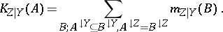 |
It may be viewed as an analogue of the true mass function for "a priori conditionals" , as it is non-negative and for any fixed value of $Y$ the sum over $Z$ equals $1$. Contrary to intuitions with probability distributions, the combination of an a priori conditional belief function with a (true) belief function by Dempster's rule need not lead to a belief function. Hence such a priori functions are poorly investigated so far (2000).
Naive case-based approach.
Currently (as of 2000), at least three naive case-based models compatible with the definition of belief function, Dempster's rule of evidence combination and Dempster 's rule of conditioning exist: the marginally correct approximation, the qualitative model and the quantitative model.
Marginally correct approximation.
This approach [a3] assumes that the belief function shall constitute lower bounds for frequencies; however, only for the marginals and not for the joint distribution. Then the reasoning process is expressed in terms of so-called Cano conditionals [a1] — a special class of a priori conditional belief functions that are everywhere non-negative. As for a general belief function, the Cano conditionals usually do not exist, they have to be calculated as an approximation to the actual a priori conditional belief function. This approach involves a modification of the reasoning mechanism, because the correctness is maintained only by reasoning forward. Depending on the reasoning direction, one needs different "Markov trees" for the reasoning engine.
Qualitative approach.
This approach [a4] is based on earlier rough set interpretations in Dempster–Shafer theory [a9], but makes a small and still significant distinction. All computations are carried out in a strictly "relational" way, i.e. indistinguishable objects in a database are merged (no object identities). The behaviour under reasoning fits strictly into the reasoning model of Dempster–Shafer theory. Factors of the hypergraph representation can be expressed by relational tables. Conditional independence is well defined. However, there is no interpretation for conditional belief functions in this model.
Quantitative approach.
The quantitative model [a5], [a11] assumes that during the reasoning process one attaches labels to objects, hiding some of their properties. There is a full agreement with the reasoning mechanism of Dempster–Shafer theory (in particular, Dempster's rule of conditioning). When combining two independent belief functions, only in the limit agreement with Dempster's rule of evidence combination can be achieved. Conditional independence and conditional belief functions are well defined. Processes have also been elaborated that, in the limit, can give rise to well-controlled graphoidally structured belief functions, and learning procedures for the discovery of graphoidal structures from data have been elaborated. The quantitative model seems to be the model best fitting for belief functions.
Subjectivist approach.
One assumes that among the elements of the set $\Omega$, called "worlds" , one world corresponds to the "actual world" . There is an agent who does not know which world is the actual world and who can only express the strength of his/her opinion (called the degree of belief) that the actual world belongs to a certain subset of $\Omega$. One such approach is the so-called transferable belief model [a10]. Besides the two already mentioned rules of Dempster (combination and conditioning), many more rules handling various sources of evidence have been added, including disjunctive rules of combination, alpha-junctions rules, cautious rules, pignistic transformation, a specialization concept, a measure of information content, canonical decomposition, concepts of confidence and diffidence, and a generalized Bayesian theorem. Predominantly, the qualitative behaviour of subjectively assigned beliefs is studied. So far (as of 2000), no attempt paralleling the subjective probability approach of B. de Finetti has been made to bridge the gap between subjective belief assignment and observed frequencies.
References
| [a1] | J. Cano, M. Delgado, S. Moral, "An axiomatic framework for propagating uncertainty in directed acyclic networks" Internat. J. Approximate Reasoning , 8 (1993) pp. 253–280 |
| [a2] | A.P. Dempster, "Upper and lower probabilities induced by a multi-valued mapping" Ann. Math. Stat. , 38 (1967) pp. 325–339 |
| [a3] | M.A. Kłopotek, S.T. Wierzchoń, "On marginally correct approximations of Dempster–Shafer belief functions from data" , Proc. IPMU'96 (Information Processing and Management of Uncertainty), Grenada (Spain), 1-5 July , II , Univ. Granada (1996) pp. 769–774 |
| [a4] | M.A. Kłopotek, S.T. Wierzchoń, "Qualitative versus quantitative interpretation of the mathematical theory of evidence" Z.W.Raś (ed.) A. Skowron (ed.) , Foundations of Intelligent Systems 7. Proc. ISMIS'97 (Charlotte NC, 15-17 Oct., 1997) , Lecture Notes in Artificial Intelligence , 1325 , Springer (1997) pp. 391–400 |
| [a5] | M.A. Kłopotek, "On (anti)conditional independence in Dempster–Shafer theory" J. Mathware and Softcomputing , 5 : 1 (1998) pp. 69–89 |
| [a6] | G. Shafer, "A mathematical theory of evidence" , Princeton Univ. Press (1976) |
| [a7] | P. Shenoy, G. Shafer, "Axioms for probability and belief-function propagation" R.D. Shachter (ed.) T.S. Levitt (ed.) L.N. Kanal (ed.) J.F. Lemmer (ed.) , Uncertainty in Artificial Intelligence , 4 , Elsevier (1990) |
| [a8] | P.P. Shenoy, "Conditional independence in valuation based systems" Internat. J. Approximate Reasoning , 109 (1994) |
| [a9] | A. Skowron, J.W. Grzymała-Busse, "From rough set theory to evidence theory" R.R. Yager (ed.) J. Kasprzyk (ed.) M. Fedrizzi (ed.) , Advances in the Dempster–Shafer Theory of Evidence , Wiley (1994) pp. 193–236 |
| [a10] | Ph. Smets, "Numerical representation of uncertainty" D.M. Gabbay (ed.) Ph. Smets (ed.) , Handbook of Defeasible Reasoning and Uncertainty Management Systems , 3 , Kluwer Acad. Publ. (1998) pp. 265–309 |
| [a11] | S.T. Wierzchoń, M.A. Kłopotek, "Modified component valuations in valuation based systems as a way to optimize query processing" J. Intelligent Information Syst. , 9 (1997) pp. 157–180 |
Dempster-Shafer theory. Encyclopedia of Mathematics. URL: http://encyclopediaofmath.org/index.php?title=Dempster-Shafer_theory&oldid=22343