Dirichlet process
The Dirichlet process provides one means of placing a probability distribution on the space of distribution functions, as is done in Bayesian statistical analysis (cf. also Bayesian approach). The support of the Dirichlet process is large: For each distribution function there is a set of distributions nearby that receives positive probability. This contrasts with a typical probability distribution on the space of distribution functions where, for example, one might place a probability distribution on the mean and variance of a normal distribution. The support in this example would be contained in the collection of normal distributions. The large support of the Dirichlet process accounts for its use in non-parametric Bayesian analysis. General references are [a4], [a5].
The Dirichlet process is indexed by its parameter, a non-null, finite measure  . Formally, consider a space
  with a collection of Borel sets
  on
on  . The random probability distribution
  has a Dirichlet process prior distribution with parameter
  , denoted by
  , if for every measurable partition
  of
of  the random vector
  has the Dirichlet distribution with parameter vector
  .
.
When a prior distribution is put on  , then for every measurable subset
  of
of  , the quantity
  is a random variable. Then
 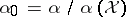 is a probability measure on
  . From the definition one sees that if
  , then
 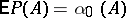 .
.
An alternative representation of the Dirichlet process is given in [a6]: Let  be independent and identically distributed
 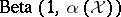 random variables, and let
  be a sequence of independent and identically distributed random variables with distribution
  , and independent of the random variables
  . Define
  , and
, and 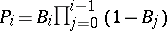 . The random distribution
  has the distribution
  . Here,
  represents the point mass at
  . This representation makes clear the fact that the Dirichlet process assigns probability one to the set of discrete distributions, and emphasizes the role of the mass of the measure
  . For example, as
  ,
,  converges to the point mass at
  (in the weak topology induced by
  ); and as
  ,
,  converges to the random distribution which is degenerate at a point
  , whose location has distribution
  .
.
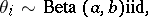
The Dirichlet process is conjugate, in that if  , and data points
  independent and identically drawn from
  are observed, then the conditional distribution of
  given
given  is
is  . This conjugation property is an extension of the conjugacy of the Dirichlet distribution for multinomial data. It ensures the existence of analytical results with a simple form for many problems. The combination of simplicity and usefulness has given the Dirichlet process its reputation as the standard non-parametric model for a probability distribution on the space of distribution functions.
An important extension of the class of Dirichlet processes is the class of mixtures of Dirichlet processes. A mixture of Dirichlet processes is a Dirichlet process in which the parameter measure is itself random. In applications, the parameter measure ranges over a finite-dimensional parametric family. Formally, one considers a parametric family of probability distributions 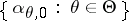 . Suppose that for every
  ,
,  is a positive constant, and let
 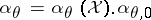 . If
. If  is a probability distribution on
  , and if, first,
  is chosen from
  , and then
  is chosen from
  , one says that the prior on
  is a mixture of Dirichlet processes (with parameter
  ). A reference for this is [a1]. Often,
  , i.e., the constants
  do not depend on
  . In this case, large values of
  indicate that the prior on
  is "concentrated around the parametric family aq,0qQ" . More precisely, as
  , the distribution of
  converges to
  , the standard Bayesian model for the parametric family
  in which
  has prior
  .
.
The Dirichlet process has been used in many applications. A particularly interesting one is the Bayesian hierarchical model, which is the Bayesian version of the random effects model. A typical example is as follows. Suppose one is studying the success of a certain type of operation for patients from different hospitals. Suppose one has  patients in hospital
  ,
,  . One might model the number of failures
  in hospital
  as a binomial distribution, with success probability depending on the hospital. And one might wish to view the
  binomial parameters as being independent and identically distributed drawn from a common distribution. The typical hierarchical model then is written as
 | (a1) |
 |
 |
Here, the  are unobserved, or latent, variables. If the distribution
  was degenerate, then the
  would be independent, so that data from one hospital would not give any information on the success rate from any other hospital. On the other hand, when
  is not degenerate, then data coming from the other hospitals provide some information on the success rate of hospital
  .
.
Consider now the problem of prediction of the number of successes for a new hospital, indexed  . A disadvantage of the model (a1) is that if the
  are independent and identically drawn from a distribution which is not a Beta, then even as
  , the predictive distribution of
  based on the (incorrect) model (a1) need not converge to the actual predictive distribution of
  . An alternative model, using a mixture of Dirichlet processes prior, would be written as
 | (a2) |
 |
 |
 |
The model (a2) does not have the defect suffered by (a1), because the support of the distribution on  is the set of all distributions concentrated in the interval
  .
.
It is not possible to obtain closed-form expressions for the posterior distributions in (a2). Computational schemes to obtain these have been developed by M. Escobar and M. West [a3] and C.A. Bush and S.N. MacEachern [a2].
The parameter  plays an interesting role. When
  is small, then, with high probability, the
  are all equal, so that, in effect, one is working with the model in which the
  are independent binomial samples with the same success probability. On the other hand, when
  is large, the model (a2) is very close to (a1).
It is interesting to note that when  is large and the distribution
  is degenerate, then the measure on
  is essentially degenerate, so that one is treating the data from the hospitals as independent. Thus, when the distribution
  is degenerate, the parameter
  determines the extent to which data from other hospitals is used when making an inference about hospital
  , and in that sense plays the role of tuning parameter in the bias-variance tradeoff of frequentist analysis.
References
| [a1] | C. Antoniak, "Mixtures of Dirichlet processes with applications to Bayesian nonparametric problems" Ann. Statist. , 2 (1974) pp. 1152–1174 |
| [a2] | C.A. Bush, S.N. MacEachern, "A semi-parametric Bayesian model for randomized block designs" Biometrika , 83 (1996) pp. 275–285 |
| [a3] | M. Escobar, M. West, "Bayesian density estimation and inference using mixtures" J. Amer. Statist. Assoc. , 90 (1995) pp. 577–588 |
| [a4] | T.S. Ferguson, "A Bayesian analysis of some nonparametric problems" Ann. Statist. , 1 (1973) pp. 209–230 |
| [a5] | T.S. Ferguson, "Prior distributions on spaces of probability measures" Ann. Statist. , 2 (1974) pp. 615–629 |
| [a6] | J. Sethuraman, "A constructive definition of Dirichlet priors" Statistica Sinica , 4 (1994) pp. 639–650 |
Dirichlet process. Encyclopedia of Mathematics. URL: http://encyclopediaofmath.org/index.php?title=Dirichlet_process&oldid=37599