Butcher series
B-series
Let  be an analytic function satisfying an ordinary differential equation
 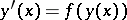 . A Butcher series for
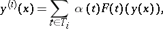
  is a series of the form
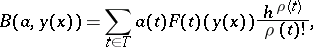 |
where  is the set of rooted trees,
  is the coefficient for the series associated with the tree
  ,
, 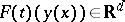 is the elementary differential associated with the tree
  ,
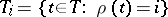
,  is a stepsize or
  -increment, and
  , often called the order of the tree
  , is the number of nodes in the tree
  . All terms will be defined below. For a more thorough discussion of Butcher series, see [a1] or [a2].
Definitions
A tree is a connected acyclic graph (cf. also Graph). A rooted tree is a tree with a distinguished node, called the root (which is drawn at the bottom of the sample trees in the Table). Two rooted trees  and
and  are isomorphic (i.e., equivalent) if and only if there is a bijection
  from the nodes of
  to the nodes of
  such that
  maps the root of
  to the root of
  and any two nodes
  and
and  are connected by an edge in
  if and only if
  and
and  are connected by an edge in
  .
.
The following bracket notation for rooted trees is very useful. Let  and
and  be the trees with zero and one node, respectively. For rooted trees
  with
with  for
for  , let
, let  be the rooted tree formed by connecting a new root to the roots of each of
  . Clearly,
 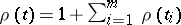 and any rooted tree formed by permuting the subtrees
  of
of  is isomorphic to
  . The rooted trees with at most four nodes are displayed in the table below.
<tbody> </tbody>
|


Using this bracket notation for rooted trees, one can recursively define elementary differentials, as follows. Let
 |
and, for  with
with  for
for  ,
,
 |
 |
where  , the
, the  th derivative of
  with respect to
  , is a multi-linear mapping.
Since  satisfies
  , it is not hard to show that
 |
where  is the
  th derivative of
  with respect to
  ,
,  , and
, and  is the number of distinct ways of labeling the nodes of
  with the integers
  such that the labels increase as you follow any path from the root to a leaf of
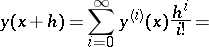
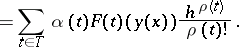
  . Consequently, one can write the Taylor series for
  as a Butcher series:
 | (a1) |
 |
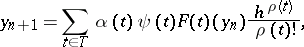
The importance of Butcher series stems from their use to derive and to analyze numerical methods for differential equations. For example, consider the  -stage Runge–Kutta formula (cf. Runge–Kutta method)
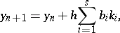 | (a2) |
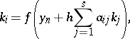 |
for the ordinary differential equation  . Let
. Let 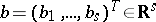 be the vector of weights and
 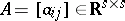 the coefficient matrix for (a2). Then it can be shown that
  can be written as the Butcher series
 | (a3) |
where the coefficients  , defined below, depend only on the rooted tree
  and the coefficients of the formula (a2).
To define  , first let
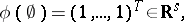 |
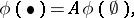 |
and then, for  with
with  for
for  , define
  recursively by
 |
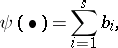
where the product of  's in the bracket is taken component-wise. Then
 |
 |
and, for  with
with  for
for  ,
,
 |
where, again, the product of  's in the bracket is taken componentwise.
Assuming that  and that
  for all trees
  of order
  , it follows immediately from (a1) and (a3) that
 |
The order of (a2) is the largest such  .
.
References
| [a1] | J.C. Butcher, "The numerical analysis of ordinary differential equations" , Wiley (1987) |
| [a2] | E. Hairer, S.P. Nørsett, G. Wanner, "Solving ordinary differential equations I: nonstiff problems" , Springer (1987) |
Butcher series. Encyclopedia of Mathematics. URL: http://encyclopediaofmath.org/index.php?title=Butcher_series&oldid=35592