Linear ordinary differential equation

An ordinary differential equation (cf. Differential equation, ordinary) that is linear in the unknown function of one independent variable and its derivatives, that is, an equation of the form

(1)

where is the unknown function and , are given functions; the number is called the order of equation (1) (below the general theory of linear ordinary differential equations is presented; for equations of the second order see also Linear ordinary differential equation of the second order).

1) If in (1) the functions are continuous on the interval , then for any numbers 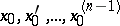and there is a unique solution of (1) defined on the whole interval and satisfying the initial conditions

The equation

(2)

is called the homogeneous equation corresponding to the inhomogeneous equation (1). If is a solution of (2) and

then . If are solutions of (2), then any linear combination

is a solution of (2). If the functions

(3)

are linearly independent solutions of (2), then for every solution of (2) there are constants such that

(4)

Thus, if (3) is a fundamental system of solutions of (2) (i.e. a system of linearly independent solutions of (2)), then its general solution is given by (4), where are arbitrary constants. For every non-singular matrix and every there is a fundamental system of solutions (3) of equation (2) such that

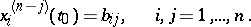For the functions (3) the determinant

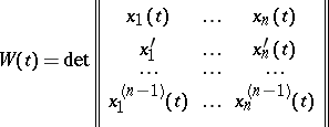is called the Wronski determinant, or Wronskian. If (3) is a fundamental system of solutions of (2), then for all . If for at least one point , then and the solutions (3) of equation (2) are linearly dependent in this case. For the Wronskian of the solutions (3) of equation (2) the Liouville–Ostrogradski formula holds:

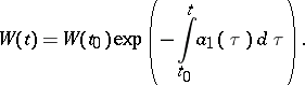The general solution of (1) is the sum of the general solution of the homogeneous equation (2) and a particular solution of the inhomogeneous equation (1), and is given by the formula

where is a fundamental system of solutions of (2) and are arbitrary constants. If a fundamental system of solutions (3) of equation (2) is known, then a particular solution of the inhomogeneous equation (1) can be found by the method of variation of constants.

2) A system of linear ordinary differential equations of order is a system

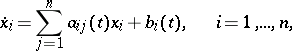or, in vector form,

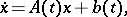(5)

where is an unknown column vector, is a square matrix of order and is a given vector function. Suppose also that and are continuous on some interval . In this case, for any and there is a unique solution of the system (5) defined on the whole interval and satisfying the initial condition .

The linear system

(6)

is called the homogeneous system corresponding to the inhomogeneous system (5). If is a solution of (6) and , then ; if are solutions, then any linear combination

is a solution of (6); if are linearly independent solutions of (6), then the vectors are linearly independent for any . If the vector functions

(7)

form a fundamental system of solutions of (6), then for every solution of (6) there are constants such that

(8)

Thus, formula (8) gives the general solution of (6). For any and any linearly independent vectors there is a fundamental system of solutions (7) of the system (6) such that

For vector functions (7) that are solutions of (6), the determinant of the matrix

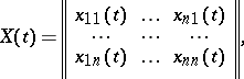(9)

where is the -th component of the -th solution, is called the Wronski determinant, or Wronskian. If (7) is a fundamental system of solutions of (6), then for all and (9) is called a fundamental matrix. If the solutions (7) of the system (6) are linearly dependent for at least one point , then they are linearly dependent for any , and in this case . For the Wronskian of the solutions (7) of the system (6) Liouville's formula holds:

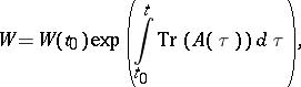where is the trace of the matrix . The matrix (9) satisfies the matrix equation . If is a fundamental matrix of the system (6), then for every other fundamental matrix of this system there is a constant non-singular matrix such that 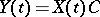. If , where is the unit matrix, then the fundamental matrix is said to be normalized at the point and the formula 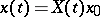gives the solution of (6) satisfying the initial condition .

If the matrix commutes with its integral, then the fundamental matrix of (6) normalized at the point is given by the formula

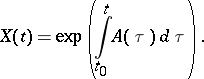In particular, for a constant matrix the fundamental matrix normalized at the point is given by the formula 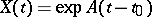. The general solution of (5) is the sum of the general solution of the homogeneous system (6) and a particular solution of (5) and is given by the formula

where is a fundamental system of solutions of (6) and are arbitrary constants. If a fundamental system of solutions (7) of the system (6) is known, then a particular solution of the inhomogeneous system (5) can be found by the method of variation of constants. If is a fundamental matrix of the system (6), then the formula

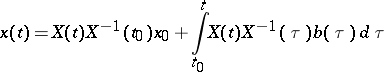gives the solution of (5) satisfying the initial condition .

3) Suppose that in the system (5) and (6) and are continuous on a half-line . All solutions of (5) are simultaneously either stable or unstable, so the system (5) is said to be stable (uniformly stable, asymptotically stable) if all its solutions are stable (respectively, uniformly stable, asymptotically stable, cf. Asymptotically-stable solution; Lyapunov stability). The system (5) is stable (uniformly stable, asymptotically stable) if and only if the system (6) is stable (respectively, uniformly stable, asymptotically stable). Therefore, in the investigation of questions on the stability of linear differential systems it suffices to consider only homogeneous systems.

The system (6) is stable if and only if all its solutions are bounded on the half-line . The system (6) is asymptotically stable if and only if

(10)

for all its solutions . The latter condition is equivalent to (10) being satisfied for solutions of the system that form a fundamental system of solutions. An asymptotically-stable system (6) is asymptotically stable in the large.

A linear system with constant coefficients

(11)

is stable if and only if all eigen values of have non-positive real parts (that is, , ), and the eigen values with zero real part may have only simple elementary divisors. The system (11) is asymptotically stable if and only if all eigen values of have negative real parts.

4) The system

(12)

where is the transposed matrix of , is called the adjoint system of the system (6). If and are arbitrary solutions of (6) and (12), respectively, then the scalar product

If and are fundamental matrices of solutions of (6) and (12), respectively, then

where is a non-singular constant matrix.

5) The investigation of various special properties of linear systems, particularly the question of stability, is connected with the concept of the Lyapunov characteristic exponent of a solution and the first method in the theory of stability developed by A.M. Lyapunov (see Regular linear system; Reducible linear system; Lyapunov stability).

6) Two systems of the form (6) are said to be asymptotically equivalent if there is a one-to-one correspondence between their solutions and such that

If the system (11) with a constant matrix is stable, then it is asymptotically equivalent to the system , where the matrix is continuous on and

(13)

If (13) is satisfied, the system is asymptotically equivalent to the system .

Two systems of the form (11) with constant coefficients are said to be topologically equivalent if there is a homeomorphism that takes oriented trajectories of one system into oriented trajectories of the other. If two square matrices and of order have the same number of eigen values with negative real part and have no eigen values with zero real part, then the systems and are topologically equivalent.

7) Suppose that in the system (6) the matrix is continuous and bounded on the whole real axis. The system (6) is said to have exponential dichotomy if the space splits into a direct sum: , , so that for every solution with the inequality

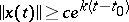holds, and for every solution with the inequality

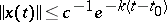holds for all and , where and are constants. For example, exponential dichotomy is present in a system (11) with constant matrix if has no eigen values with zero real part (such a system is said to be hyperbolic). If the vector function is bounded on the whole real axis, then a system (5) having exponential dichotomy has a unique solution that is bounded on the whole line .

References

[1]	I.G. Petrovskii, "Ordinary differential equations" , Prentice-Hall (1966) (Translated from Russian)
[2]	L.S. Pontryagin, "Ordinary differential equations" , Addison-Wesley (1962) (Translated from Russian)
[3]	V.I. Arnol'd, "Ordinary differential equations" , M.I.T. (1973) (Translated from Russian)
[4]	A.M. [A.M. Lyapunov] Liapounoff, "Problème général de la stabilité du mouvement" , Princeton Univ. Press (1947) (Translated from Russian) (Reprint, Kraus, 1950)
[5]	B.P. Demidovich, "Lectures on the mathematical theory of stability" , Moscow (1967) (In Russian)
[6]	B.F. Bylov, R.E. Vinograd, D.M. Grobman, V.V. Nemytskii, "The theory of Lyapunov exponents and its applications to problems of stability" , Moscow (1966) (In Russian)
[7]	P. Hartman, "Ordinary differential equations" , Birkhäuser (1982)

Comments

If in (6) is periodic with period , the fundamental matrix is of the form

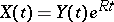with a matrix with -periodic coefficients and a constant matrix, see Floquet theory for more details.

References

[a1]	R.E. Bellman, "Stability theory of differential equations" , McGraw-Hill (1953)
[a2]	E.A. Coddington, N. Levinson, "Theory of ordinary differential equations" , McGraw-Hill (1955) pp. Chapts. 13–17