Elliptic functions (cf. Elliptic function) resulting from the direct inversion of elliptic integrals (cf. Elliptic integral) in Legendre normal form. This inversion problem was solved in 1827 independently by C.G.J. Jacobi and, in a slightly different form, by N.H. Abel. Jacobi's construction is based on an application of theta-functions (cf. Theta-function).
Let  be a complex number with
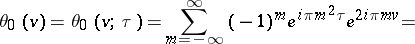
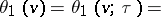
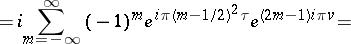
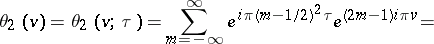
  . The Jacobi theta-functions
  ,
,  ,
,  , and
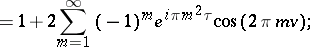
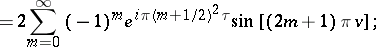
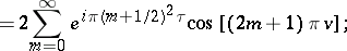
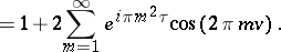
, and  are represented by the following series in the complex variable
  , which converge absolutely and uniformly on compact sets:
These series converge fairly rapidly. The notation  ,
,  ,
,  ,
,  goes back to r conditions','../w/w097460.htm','Weierstrass point','../w/w097490.htm','Weierstrass theorem','../w/w097510.htm','Weierstrass representation of a minimal surface','../w/w130040.htm')" style="background-color:yellow;">K. Weierstrass.
  is often written
  , and there are other systems of notation. Jacobi used the notation
  ,
,  ,
,  , and
, and  , where
  .
.
All Jacobi theta-functions are entire transcendental functions of the complex variable  ;
;  is an odd function, and the other functions
  ,
,  and
and  are even.
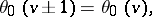
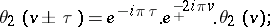
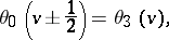
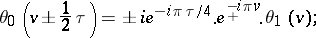
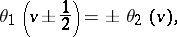
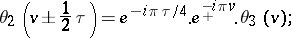
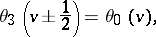
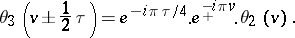
The following periodicity relations hold:
These imply that the theta-functions are elliptic Hermite functions of the third kind (cf. also Hermite function).
The various theta-functions are connected by the following transformation formulas:
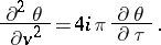
All four theta-functions satisfy one and the same differential equation (the heat equation):
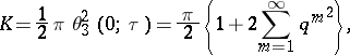
The zero arguments of the theta-functions,  ,
,  ,
,  ,
,  are important; here
  . The relations between them are:
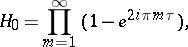
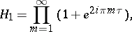
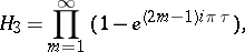
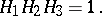
In particular,
where
The function  has simple zeros at
  ;
;  at
at  ;
;  at
at  ; and
; and  at
at  ;
;  .
.
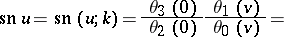
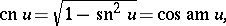
It is clear from the periodicity relations that certain ratios of theta-functions are elliptic functions in the proper sense. The basic Jacobi elliptic functions are:  (sine amplitude),
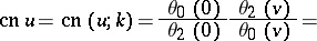
  (cosine amplitude) and
  (delta amplitude). This notation was introduced by C. Gudermann (1838). The terminology stems from the old, and outdated, notation of Jacobi:
  ,
,  ,
,  .
.
The new variable  is connected with
  by
by  . Denoting the modulus of the elliptic functions by
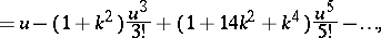
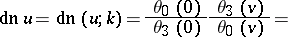
  , the Jacobi elliptic functions can be expressed in terms of theta-functions, or by means of power series that converge in a neighbourhood of the origin, as follows:
A convenient notation for inverses and ratios was introduced by J. Glaisher (1882):
The Jacobi elliptic functions  ,
,  and
and  are elliptic functions of the second order with the following periods:
  and
and  for
for  ;
;  and
and  for
for  ; and
; and  and
and  for
for  , where
  and
and  are the values of the complete elliptic integrals of the first kind, and
  is called the complementary modulus of the elliptic functions. The Jacobi elliptic functions have only simple poles, located at
  ;
;  .
.
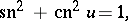
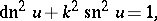
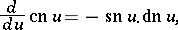
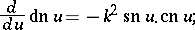
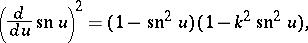
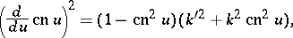
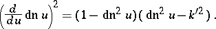
The three Jacobi elliptic functions are connected by the relations:
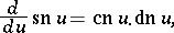
and by the differential equations:
The addition theorems for Jacobi elliptic functions are:
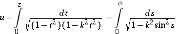
The connection between Jacobi elliptic functions and elliptic integrals is as follows. If
is an elliptic integral of the first kind in Legendre normal form, then its inverse is  ; this constitutes the starting point of the Jacobi theory. The variable
  is an infinitely-valued function of
  , and is called the amplitude of the elliptic integral
  ,
,
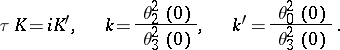
The main relations between the constants are:
In applied problems the modulus  is usually known and very often the normal case
  holds, or the complementary modulus
  ,
,  , is given. It is required to find
  ,
,  , and
, and  or
or  . By setting
  , where
  , one has
  . To find
  the following series, which converges rapidly if
  , is used:
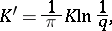
The numbers  and
and  of the complete elliptic integrals are determined by the formulas
or are found from tables.
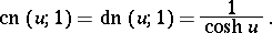
When  or
or  the Jacobi elliptic functions degenerate into trigonometric or hyperbolic functions, respectively:
Theoretically, a simpler construction of the theory of elliptic functions was given by Weierstrass (1862–1863) (see Weierstrass elliptic functions). For a given  ,
,  , the Weierstrass invariants
  are found from, for example, the formulas:
  ,
,  ,
,  , and then
  and
and  can be found. The half-periods are defined by
  and
and  ; these enable one to calculate all the remaining quantities related to the Weierstrass elliptic functions.
References
| [1a] | C.G.J. Jacobi, "Fundamenta nova theoriae functionum ellipticarum" , Königsberg (1829) |
| [1b] | C.G.J. Jacobi, "Fundamenta nova theoriae functionum ellipticarum" , Gesammelte Werke , 1 , Chelsea, reprint (1969) pp. 49–239 |
| [2] | N.I. Akhiezer, "Elements of the theory of elliptic functions" , Amer. Math. Soc. (1990) (Translated from Russian) |
| [3] | A. Hurwitz, R. Courant, "Vorlesungen über allgemeine Funktionentheorie und elliptische Funktionen" , 1 , Springer (1964) pp. Chapt.8 |
| [4] | E.T. Whittaker, G.N. Watson, "A course of modern analysis" , Cambridge Univ. Press (1952) pp. Chapt. 6 |
| [5] | A. Enneper, "Elliptische Funktionen. Theorie und Geschichte" , Halle (1890) |
| [6] | J. Tannéry, J. Molk, "Eléments de la théorie des fonctions elliptiques" , 1–2 , Chelsea, reprint (1972) |
| [7] | A.M. Zhuravskii, "Handbook on elliptic functions" , Moscow-Leningrad (1941) (In Russian) |
| [8] | E. Jahnke, F. Emde, F. Lösch, "Tafeln höheren Funktionen" , Teubner (1966) |
References
| [a1] | D. Mumford, "Tata lectures on Theta" , 1–2 , Birkhäuser (1983–1984) |
| [a2] | A. Weil, "Elliptic functions according to Eisenstein and Kronecker" , Springer (1976) |
| [a3] | F. Bowman, "Introduction to elliptic functions with applications" , Dover, reprint (1961) |
| [a4] | J.-i. Igusa, "Theta functions" , Springer (1972) |
| [a5] | H. Hancock, "Theory of elliptic functions" , Dover, reprint (1958) |