Hopf invariant

An invariant of a homotopy class of mappings of topological spaces. It was first defined by H. Hopf ([1], [2]) for mappings of spheres .

Let be a continuous mapping. By transition, if necessary, to a homotopic mapping, one may assume that this mapping is simplicial with respect to certain triangulations of the spheres and . Then the Hopf invariant is defined as the linking coefficient of the -dimensional disjoint submanifolds and in for any distinct .

The mapping determines an element , and the image of the element under the homomorphism

coincides with the Hopf invariant (here is the Hurewicz homomorphism) [3].

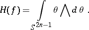
Suppose now that is a mapping of class and that a form is a generator of the integral cohomology group . For such a form one may take, for example, , where is the volume element on in some metric (for example, in the metric given by the imbedding ), and is the volume of the sphere . Then the form is closed and it is exact because the group is trivial. Thus, for some form . A formula for the computation of the Hopf invariant is (see [4]):

The definition of the Hopf invariant can be generalized (see [5], [6]) to the case of mappings for . In this case there is a decomposition

(*)

where

is the homomorphism induced by the projection . Let be the mapping given by contracting the equator of the sphere to a point. Then the Hopf invariant is defined as the homomorphism

under which is transformed to the projection of the element onto the direct summand in the decomposition (*). Since , for one obtains the usual Hopf invariant. The generalized Hopf invariant is defined as the composite of the homomorphisms

where is the projection of the group onto the direct summand , and the homomorphisms and are described above. For the Hopf–Whitehead invariant and the Hopf–Hilton invariant are connected by the relation , where is the suspension homomorphism (see [6]).

Let be a mapping and let be its cylinder (cf. Mapping cylinder). Then the cohomology space has as homogeneous -basis a pair with and . Here the relation holds (see [7]). If is odd, then (because multiplication in cohomology is skew-commutative).

There is (see [8]) a generalization of the Hopf–Steenrod invariant in terms of a generalized cohomology theory (cf. Generalized cohomology theories). Let be the semi-exact homotopy functor in the sense of Dold (see [9]), given on the category of finite CW-complexes and taking values in a certain Abelian category . Then the mapping of complexes determines an element , where is the set of morphisms in . The Hopf–Adams invariant is defined when and , where is the corresponding suspension mapping. In this case the sequence of cofibrations

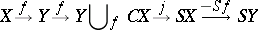corresponds to an exact sequence in :

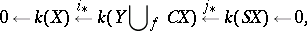which determines the Hopf–Adams–Steenrod invariant .

In the case of the functor taking values in the category of modules over the Steenrod algebra modulo 2, one obtains the Hopf–Steenrod invariant of a mapping for (see [7]). The cohomology space has as -basis a pair with and , and then

The Hopf invariant modulo (where is a prime number) is defined as the composite of the mappings

where is the localization by of the pair of spaces (see [10]). Let

be the suspension homomorphism. Then (see [10]). The Hopf invariant can also be defined in terms of the Stiefel numbers (cf. Stiefel number) (see [11]): If is a closed equipped manifold and if , then the characteristic Stiefel–Whitney number of the normal bundle is the same as the Hopf invariant of the mapping that is a representative of the class of equipped cobordisms of .

The Adams–Novikov spectral sequence makes it possible to construct higher Hopf invariants. Namely, one defines inductively the invariants and (see [12]). From the form of the differentials of this spectral sequence it follows that

(where is the ring of complex point cobordisms); therefore, for , the invariants lie in and are called the Hopf–Novikov invariants. For one obtains the Adams invariant.

The values that a Hopf invariant can take are not arbitrary. For example, for a mapping the Hopf invariant is always 0. The Hopf invariant modulo , , is trivial, except when , and , . On the other hand, for any even number there exists a mapping with Hopf invariant ( is arbitrary). For there exists mappings with Hopf invariant 1.

References

[1]	H. Hopf, "Ueber die Abbildungen der dreidimensionalen Sphäre auf die Kügelfläche" Math. Ann. , 104 (1931) pp. 639–665
[2]	H. Hopf, "Ueber die Abbildungen von Sphären niedriger Dimension" Fund. Math. , 25 (1935) pp. 427–440
[3]	J.-.P. Serre, "Groupes d'homotopie et classes de groupes abéliens" Ann. of Math. , 58 : 2 (1953) pp. 258–294
[4]	J.H.C. Whitehead, "An expression of the Hopf invariant as an integral" Proc. Nat. Acad. Sci. USA , 33 (1937) pp. 117–123
[5]	J.H.C. Whitehead, "A generation of the Hopf invariant" Ann. of Math. (2) , 51 (1950) pp. 192–237
[6]	P. Hilton, "Suspension theorem and generalized Hopf invariant" Proc. London. Math. Soc. (3) , 1 : 3 (1951) pp. 462–493
[7]	N. Steenrod, "Cohomologies invariants of mappings" Ann. of Math. (2) , 50 (1949) pp. 954–988
[8]	J. Adams, "On the groups " Topology , 5 (1966) pp. 21–71
[9]	A. Dold, "Halbexakte Homotopiefunktoren" , Springer (1966)
[10]	D. Husemoller, "Fibre bundles" , McGraw-Hill (1966)
[11]	R.E. Stong, "Notes on cobordism theory" , Princeton Univ. Press (1968)
[12]	S.P. Novikov, "The methods of algebraic topology from the view point of cobordism theories" Math. USSR-Izv. , 4 : 1 (1967) pp. 827–913 Izv. AKad. Nauk SSSR Ser. Mat. , 31 : 4 (1967) pp. 855–951
[13]	J.F. Adams, "On the non-existence of elements of Hopf invariant one" Ann. of Math. , 72 (1960) pp. 20–104