Extremal problems, numerical methods

Methods of computational mathematics that are applied to find the extrema (maxima or minima) of functions and functionals.

The numerical solution of extremal problems considered in infinite-dimensional function spaces (for example, problems of optimal control by means of processes described by ordinary or partial differential equations) can be obtained by using appropriate generalizations of many methods of mathematical programming developed for problems of minimization or maximization of functions of finitely many variables. In this context it is very important to make the correct choice of a suitable function space in which a concrete problem should be considered. Such a space is usually chosen by taking into account physical considerations, properties of admissible controls, properties of the solutions of the corresponding initial-boundary value problems for a fixed control, etc.

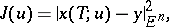
For example, the problem of optimal control consisting of the minimization of the functional

(1)

under the conditions

(2)

(3)

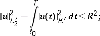
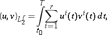
is usually considered in the function space . Here , , , , , and are given functions, and known moments in time, , is a given initial point, is a given set in the Euclidean space for every , and is the Hilbert space of -dimensional vector functions , , where each function is, together with its square, Lebesgue integrable over ; the inner product of two functions and in this space is defined by

and the norm by

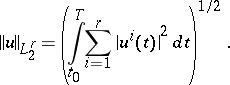For a specific degree of smoothness of the functions and the increment of the functional (1) can be represented in the form

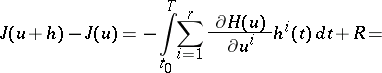(4)

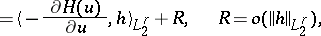where

(5)

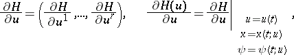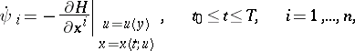
is the solution of the problem (2) for , and is the solution of the adjoint problem

(6)

(7)

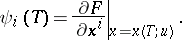
Formula (4) implies that the functional (1) is differentiable in and that its gradient is the vector function

(8)

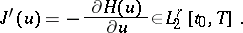
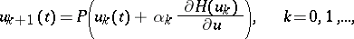
Hence, (1)–(3) can be solved by applying various methods that use the gradient of the functional. For one may apply the gradient method

If , where and are given functions in , then it is possible to apply the method of gradient projection:

where

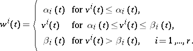The parameter can be chosen from the condition . The methods of the conditional gradient, dual gradients, etc. (see [4]–[6] and [11]) can be adapted for the problem (1)–(3) analogously. If this problem is considered under the additional restrictions

(9)

where is a given set in , then these restrictions can be taken into account by using the method of penalty functions (cf. Penalty functions, method of). For example, if

then as a penalty function one may take

and (1)–(3), (9) is replaced by the problem of minimizing the functional under the conditions (2) and (3), where is the penalty coefficient and .

Other methods for solving (1)–(3), (9) are based on Pontryagin's maximum principle and on dynamic programming (see Pontryagin maximum principle; Dynamic programming and Variational calculus, numerical methods of).

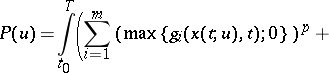
The problem of minimizing a quadratic functional subject to a system of linear ordinary differential equations or linear partial differential equations can be solved by applying the method of moments (see [3] and [8]). This method is described below when applied to the problem of minimizing the functional

(10)

where is the solution of the problem

(11)

and the controls 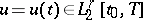are such that

(12)

here , and are given matrices of order , and , respectively, with piecewise-continuous entries on the interval , , are given points, , and is the inner product in . From the rule of Lagrange multipliers it follows that the control is optimal in the problem (10)–(12) if and only if there is a number (the Lagrange multiplier for the constraint (12)) such that

(13)

(14)

here for . Formulas (5)–(8) imply that the gradient of the functional (10) in has the form

where is the solution of the problem

(15)

(16)

here and are the transposed matrices of and , respectively. Then condition (13) becomes

(17)

Condition (16) is equivalent to

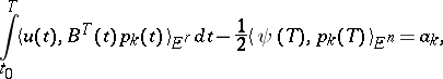(18)

for , where

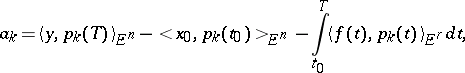and is the solution of the system (15) satisfying (a unit vector). Hence, the optimal control in the problem (10)–(12) is determined by solving the system (14), (15), (17), (18) relative to the functions and and the number . If , then , and (18) reduces to the problem of moments (see Moment problem): To find a function , knowing

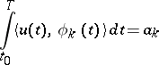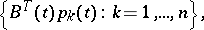
with respect to the system , .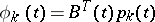

System (14), (15), (17), (18) is a generalized moment problem for (10)–(12) with (see [3] and [8]).

Any solution of (15) is uniquely representable in the form

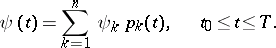(19)

System (15), (17), (18) has a solution , for any fixed , and among all its solutions there is a unique one such that has the form

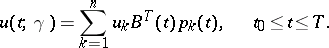(20)

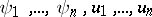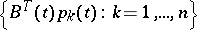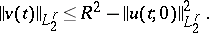
To find and one substitutes (19) and (20) in (17) and (18) and obtains a system of linear algebraic equations with respect to , from which are determined uniquely and non-uniquely if the system is linearly dependent. In the practical solution of the problem (10)–(12) it is advisable to set and from the beginning and to use (18) to determine of the form (20). Next, it must be checked that 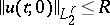. If this inequality holds, then is the optimal control of (10)–(12) with minimal norm among all optimal controls; the set of all optimal controls in this case consists of controls of the form

where belongs to the orthogonal complement in of the linear span of the system of functions

If 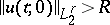, then for the solutions and of the form (19) and (20), respectively, are found from (17) and (18), and is found from the equation

(21)

The function of the variable is continuous and strictly decreasing for , and ; therefore, the desired is determined uniquely from (21). The control is optimal for the problem (10)–(12); for this problem has no other optimal controls.

The method of moments is also applicable for the solution of the high-speed problem for the system (11) and other linear systems (see [3] and [8]).

The above methods are also widely used for the numerical solution of problems of optimal control by means of processes described by partial differential equations.

The numerical realizations of many methods for solving problems of optimal control are based on the use of some technique for the approximate solution of the intervening initial-boundary value problems (see Boundary value problem, numerical methods for partial differential equations) and of approximate computations of integrals (see Integration, numerical). As a result, the original problem of optimal control is replaced by a family of approximate problems depending on some parameters (for example, on the steps of the difference grid). About questions regarding the construction of approximate problems and the investigation of their convergence, see [5].

Large classes of extremal problems are ill posed (see Ill-posed problems) and their solution requires the use of a regularization method (see [5] and [3]).

References

[1]	V.M. Alekseev, V.M. Tikhomirov, S.V. Fomin, "Optimal control" , Consultants Bureau (1987) (Translated from Russian)
[2]	I.V. Beiko, B.N. Bublik, P.N. Zin'ko, "Methods and algorithms for the solution of optimization problems" , Kiev (1983) (In Russian)
[3]	A.G. Butkovskii, "Methods of control by means of systems with distributed parameters" , Moscow (1975) (In Russian)
[4]	F.P. Vasil'ev, "Numerical method for solving extremal problems" , Moscow (1980) (In Russian)
[5]	F.P. Vasil'ev, "Methods for solving extremal problems" , Moscow (1981) (In Russian)
[6]	Yu.G. Evtushenko, "Numerical optimization techniques" , Optim. Software (1985) (Translated from Russian)
[7]	A.I. Egorov, "Optimal control by means of thermal and diffusion processes" , Moscow (1978) (In Russian)
[8]	N.N. Krasovskii, "Theory of control by motion" , Moscow (1968) (In Russian)
[9]	J.-L. Lions, "Optimal control of systems governed by partial differential equations" , Springer (1971) (Translated from French)
[10]	B.T. Polyak, "Introduction to optimization" , Moscow (1983) (In Russian)
[11]	J. Céa, "Lectures on optimization: theory and algorithms" , Springer (1978)
[12]	T.K. Sirazetdinov, "Optimization of systems with distributed parameters" (1977) (In Russian)
[13]	A.N. Tikhonov, V.I. [V.I. Arsenin] Arsenine, "Solutions of ill-posed problems" , Winston (1977) (Translated from Russian)
[14]	R.P. Fedorenko, "Approximate solution of problems of optimal control" , Moscow (1978) (In Russian)
[15]	I. Ekeland, R. Téman, "Analyse convexe et problèmes variationnels" , Dunod (1974)

Comments

Constraints of the kind or are usually referred to as state constraints. Among the methods available for the numerical solution of optimal control problems, a distinction can be made between direct and indirect methods. With direct methods the optimal control problem is treated directly as a minimization problem, i.e. the method is started with an initial approximation of the solution, which is iteratively improved by minimizing the objective functional (cf. Objective function) (augmented with a "penalty" term) along the direction of search. The direction of search is obtained via linearization of the problem. With indirect methods the optimality conditions, which must hold for a solution of the optimal control problem, are used to derive a multi-point boundary value problem. Solutions of the optimal control problem will also be solutions of this multi-point boundary value problem and hence the numerical solution of the multi-point boundary value problem yields a candidate for the solution of the optimal control problem.

Most direct methods are of the gradient type, i.e. they are function space analogues of the well-known gradient method for finite-dimensional non-linear programming problems [a1]. These methods can be extended to Newton-like methods [a1], [a2] (cf. Newton method). As indicated in the main article above, state constraints can be treated via a penalty-function approach. Numerical results, however, indicate that this approach yields an inefficient and inaccurate method for the solution of state-constrained optimal control problems [a3]. Another way to treat state constraints is via a slack-variable transformation technique, using quadratic slack variables [a4].

A well-known indirect method is the one based on the numerical solution of the multi-point boundary value problem using multiple shooting [a3], [a5] (cf. Shooting method). For optimal control problems with state constraints, the right-hand side of the differential equation of the multi-point boundary value problem will, in general, be discontinuous at junction points, i.e. points where an inequality constraint changes from active to inactive or vice versa. These discontinuities require special attention [a1].

In general, the properties of direct and indirect methods are somewhat complementary. Direct methods tend to have a relatively large region of convergence and tend to be relatively inaccurate, whereas indirect methods generally have a relatively small region of convergence and tend to be relatively accurate.

References

[a1]	A.E. Bryson, Y.-C. Ho, "Applied optimal control" , Hemisphere (1975)
[a2]	E.R. Edge, W.F. Powers, "Function-space quasi-Newton algorithms for optimal control problems with bounded controls and singular arcs" J. Optimization Theory and Appl. , 20 (1976) pp. 455–479
[a3]	K.H. Well, "Uebungen zu den optimale Steuerungen" , Syllabus of the course "Optimierungsverfahren" of the Carl Cranz Geselschaft , Oberpfaffenhofen, FRG (1983)
[a4]	D.H. Jacobson, M.M. Lele, "A transformation technique for optimal control problems with a state variable constraint" IEEE Trans. Automatic Control , 14 : 5 (1969)
[a5]	H. Maurer, "An optimal control problem with bounded state variables and control appearing linearly" SIAM J. Control Optimization , 15 (1977) pp. 345–362
[a6]	D.P. Bertsekas, "Constrained optimization and Lagrange multiplier methods" , Acad. Press (1982)
[a7]	P.L. Falb, J.L. de Jong, "Some successive approximation methods in control and oscillation theory" , Acad. Press (1969)