Cubature formula

A formula for the approximate calculation of multiple integrals of the form

The integration is performed over a set in the Euclidean space , . A cubature formula is an approximate equality

(1)

The integrand is written as the product of two functions: the first, , is assumed to be fixed for each specific cubature formula and is known as a weight function; the second, , is assumed to belong to some fairly broad class of functions, e.g. continuous functions such that the integral exists. The sum on the right-hand side of (1) is called a cubature sum; the points are known as the interpolation points (knots, nodes) of the formula, and the numbers as its coefficients. Usually , though this condition is not necessary. In order to compute the integral via formula (1), one need only calculate the cubature sum. If formula (1) and the sum on its right-hand side are known as a quadrature formula and sum (see Quadrature formula).

Let be a multi-index, where the are non-negative integers; let ; and let be a monomial of degree in variables; let

be the number of monomials of degree at most in variables; let , be an ordering of all monomials such that monomials of lower degree have lower subscript while the monomials of equal degree have been ordered arbitrarily, e.g. in lexicographical order. In this enumeration , and the , , include all monomials of degree at most . Let be a polynomial of degree . The set of points in the complex space satisfying the equation is known as an algebraic hypersurface of degree .

One way to construct cubature formulas is based on algebraic interpolation. The points , , are so chosen that they do not lie on any algebraic hypersurface of degree or, equivalently, they are chosen such that the Vandermonde matrix

is non-singular. The Lagrange interpolation polynomial for a function with knots has the form

where is the polynomial of the influence of the -th knot: ( is the Kronecker symbol). Multiplying the approximate equality by and integrating over leads to a cubature formula of type (1) with and

(2)

The existence of the integrals (2) is equivalent to the existence of the moments of the weight function, , . Here and below it is assumed that the required moments of exist. A cubature formula (1) which has knots not contained in any algebraic hypersurface of degree and with coefficients defined by (2), is called an interpolatory cubature formula. Formula (1) has the -property if it is an exact equality whenever is a polynomial of degree at most ; an interpolatory cubature formula has the -property. A cubature formula (1) with knots which has the -property is an interpolatory formula if and only if the matrix

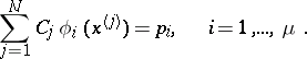
has rank . This condition holds when , so that a quadrature formula with knots that has the -property is an interpolatory formula. The actual construction of an interpolatory cubature formula reduces to a selection of the knots and a calculation of the coefficients. The coefficients are determined by the linear algebraic system of equations

which is simply the mathematical expression of the statement that (1) (with ) is exact for all monomials of degree at most . The matrix of this system is precisely ().

Now suppose it is necessary to construct a cubature formula (1) with the -property, but with less than knots. Since this cannot be done by merely selecting the coefficients, not only the coefficients but also the knots are unknowns in (1), giving unknowns in total. Since the cubature formula must have the -property, one obtains equations

(3)

It is natural to require the number of unknowns to coincide with the number of equations: . This equation gives a tentative estimate of the number of knots. If is not an integer, one puts , where denotes the integer part of . A cubature formula with this number of knots need not always exist. If it does exist, its number of knots is times the number of knots of an interpolatory cubature formula. In that case, however, the knots themselves and the coefficients are determined by the non-linear system of equations (3). In the method of undetermined parameters, one constructs a cubature formula by trying to give it a form that will simplify the system (3). This can be done when and have symmetries. The positions of the knots are taken compatible with the symmetry of and , and in that case symmetric knots are assigned the same coefficients. The simplification of the system (3) involves a certain risk: While the original system (3) may be solvable, the simplified system need not be.

Example. Let , . One is asked to construct a cubature formula with the -property; , , and 12 knots. The knots are located as follows. The first group of knots consists of the intersection points of the circle of radius , centred at the origin, with the coordinate axes. The second group consists of the intersection points of the circle of radius , also centred at the origin, with the straight lines . The third group is constructed similarly, with radius denoted by . The coefficients assigned to knots of the same group are identical and are denoted by for knots of the first, second and third group, respectively. This choice of knots and coefficients implies that the cubature formula will be exact for monomials in which at least one of or is odd. For the cubature formula to possess the -property, it will suffice to ensure that it is exact for , , , , , . This yields a non-linear system of six equations in the six unknowns , . Solving this system, one obtains a cubature formula with positive coefficients and with knots lying in .

Let be a finite subgroup of the group of orthogonal transformations of the space which leave the origin fixed. A set and a function are said to be invariant under if and for and any . The set of points of the form , where is a fixed point of and runs through all elements of , is known as the orbit containing . A cubature formula (1) is said to be invariant under if and are invariant under and if the set of knots is a union of orbits, with knots belonging to the same orbit being assigned identical coefficients. Examples of sets invariant under are the entire space , and any ball or sphere centred at the origin; if is the group of transformations of a regular polyhedron onto itself, then is also invariant. Thus, one can speak of invariant cubature formulas when is , a ball, a sphere, a cube or any regular polyhedron, and when is any function invariant under , e.g. , where .

Theorem 1) A cubature formula which is invariant under possesses the -property if and only if it is exact for all polynomials of degree at most which are invariant under (see [5]). The method of undetermined coefficients may be defined as the method of constructing invariant cubature formulas possessing the -property. In the above example, the role of the group may be played by the symmetry group of the square. Theorem 1 is of essential importance in the construction of invariant cubature formulas.

For simple domains of integration, such as a cube, a simplex, a ball, or a sphere, and for the weight , one can construct cubature formulas by repeatedly using quadrature formulas. For example, when is the cube, one may use the Gauss quadrature formula with knots and coefficients to obtain a cubature formula

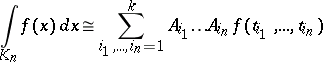with knots; this is exact for all monomials such that , , and in particular for all polynomials of degree at most . The number of knots of such cubature formulas increases rapidly, a fact which limits their applicability.

Throughout the sequel it will be assumed that the weight function is of fixed sign, say

(4)

The fact that the coefficients of a cubature formula with such a weight function are positive, is a valuable property of the formula.

Theorem 2) If the domain of integration is closed and satisfies (4), there exists an interpolatory cubature formula (1) possessing the -property, , with positive coefficients and with knots in . The question of actually constructing such a formula is as yet open.

Theorem 3) If a cubature formula with a weight satisfying (4) has real knots and coefficients and possesses the -property, then at least of its coefficients are positive, where is the integer part of . Under the assumptions of Theorem 3, the number is a lower bound for the number of knots:

This inequality remains valid without the assumption that and are real.

Regarding cubature formulas with the -property, one is particularly interested in those having a minimum number of knots. When it is easy to find such formulas for any , arbitrary and ; the minimum number of knots is precisely the lower bound : It is equal to 1 in the first case, and to in the second. When , the minimum number of knots depends on the domain and the weight. For example, if , the domain is centrally symmetric, and if , the number of knots is ; for a simplex and , it is .

By virtue of (4),

(5)

is a scalar product in the space of polynomials. Let be the vector space of polynomials of degree which are orthogonal in the sense of (5) to all polynomials of degree at most . This space has dimension — the number of monomials of degree . Polynomials in are called orthogonal polynomials for and .

Theorem 4) There exists a cubature formula (1) possessing the -property and having knots (the lower bound) if and only if the knots are the common roots of all orthogonal polynomials for and of degree .

Theorem 5) If orthogonal polynomials of degree have finite and pairwise distinct common roots, these roots can be chosen as knots for a cubature formula (1) possessing the -property.

The error of a cubature formula (1) in which and is bounded is defined by

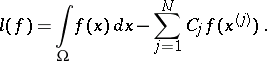Let be a Banach space of functions such that is a linear functional on . The norm of the functional characterizes the quality of a given cubature formula for all functions of . Another approach to the construction of cubature formulas is based on minimizing as a function of the knots and the coefficients of the (unknown) cubature formula (with only the number of knots fixed). Implementation of this approach, however, involves difficulties even for . Important results for any have been obtained by S.L. Sobolev [4]. The question of minimizing as a function of the coefficients for a given set of knots has been solved completely; the problem of choosing the knots is based on the assumption that they form a parallelepipedal grid and that the minimization depends exclusively on the parameters of this grid. The space , in particular, may be , where , and in that case the desired cubature formula is assumed to be exact for all polynomials of degree at most .

References

[1]	N.M. Krylov, "Approximate calculation of integrals" , Macmillan (1962) (Translated from Russian)
[2]	V.I. Krylov, L.T. Shul'gina, "Handbook on numerical integration" , Moscow (1966) (In Russian)
[3]	A.H. Stroud, "Approximate calculation of multiple integrals" , Prentice-Hall (1971)
[4]	S.L. Sobolev, "Introduction to the theory of cubature formulas" , Moscow (1974) (In Russian)
[5]	S.L. Sobolev, "Formulas for mechanical cubature on the surface of a sphere" Sibirsk. Mat. Zh. , 3 : 5 (1962) pp. 769–796 (In Russian)
[6]	I.P. Mysovskikh, "Interpolatory cubature formulas" , Moscow (1981) (In Russian)

Comments

The polynomial "of the influence of the j-th knot" (i.e. defined by ) is also called the basic Lagrangian (for ).

The "m-property" is also known in Western literature as the degree of precision; i.e. a cubature formula has the -property if it has degree of precision .

Reference [a1] is both an excellent introduction as well as an advanced treatment of cubature formulas.

References

[a1]	H. Engels, "Numerical quadrature and cubature" , Acad. Press (1980)
[a2]	P.J. Davis, P. Rabinowitz, "Methods of numerical integration" , Acad. Press (1984)