Difference between revisions of "Kolmogorov test"
(refs format) |
(picture remake) |
||
| Line 45: | Line 45: | ||
and <img align="absmiddle" border="0" src="https://www.encyclopediaofmath.org/legacyimages/k/k055/k055760/k05576036.png" /> is the [[Variational series|variational series]] (or set of order statistics) constructed from the sample <img align="absmiddle" border="0" src="https://www.encyclopediaofmath.org/legacyimages/k/k055/k055760/k05576037.png" />. The Kolmogorov test has the following geometric interpretation (see Fig.). | and <img align="absmiddle" border="0" src="https://www.encyclopediaofmath.org/legacyimages/k/k055/k055760/k05576036.png" /> is the [[Variational series|variational series]] (or set of order statistics) constructed from the sample <img align="absmiddle" border="0" src="https://www.encyclopediaofmath.org/legacyimages/k/k055/k055760/k05576037.png" />. The Kolmogorov test has the following geometric interpretation (see Fig.). | ||
| − | < | + | <center><asy> |
| − | + | srand(2014011); | |
| + | |||
| + | import stats; | ||
| + | |||
| + | int size = 13; | ||
| + | real [] sample = new real[size+1]; | ||
| + | real lambda = 1.3/size; | ||
| + | real width = 2.0; | ||
| + | |||
| + | for (int k=0; k<size; ++k) { | ||
| + | sample[k] = Gaussrand(); | ||
| + | } | ||
| + | sample[size] = 10; | ||
| + | |||
| + | sample = sort(sample); | ||
| + | |||
| + | // for (real x : sample ) { | ||
| + | // write(x); | ||
| + | // } | ||
| + | |||
| + | real x0 = -10; | ||
| + | int k = 0; | ||
| + | for (real x : sample ) { | ||
| + | filldraw( box( (x0,k/size-lambda), (x,k/size+lambda) ), rgb(0.8,0.8,0.8) ); | ||
| + | draw( (x0,k/size-lambda)..(x,k/size-lambda), currentpen+1.5 ); | ||
| + | draw( (x0,k/size)..(x,k/size), currentpen+1.5 ); | ||
| + | draw( (x0,k/size+lambda)..(x,k/size+lambda), currentpen+1.5 ); | ||
| + | k += 1; | ||
| + | x0 = x; | ||
| + | draw( (x,(k-1)/size-lambda)..(x,k/size+lambda) ); | ||
| + | } | ||
| + | |||
| + | clip( box((-width,-0.005),(width,1.005)) ); | ||
| + | |||
| + | draw ((-width,0)--(width,0),Arrow); | ||
| + | draw ((0,-0.1)--(0,1.3),Arrow); | ||
| + | draw ((-width,1)--(width,1)); | ||
| + | |||
| + | draw ((sample[2],0)..(sample[2],2/size)); | ||
| + | draw ((sample[size-1],0)..(sample[size-1],0.48), dashed); | ||
| + | draw ((sample[size-1],0.7)..(sample[size-1],1-1/size), dashed); | ||
| + | |||
| + | label("$x$",(width,0),S); | ||
| + | label("$y$",(0,1.3),W); | ||
| + | label("$0$",(0,0),SW); | ||
| + | label("$1$",(0,1),NE); | ||
| + | |||
| + | label("$X_{(1)}$",(sample[0],0),S); | ||
| + | label("$X_{(2)}$",(sample[1],0),S); | ||
| + | label("$X_{(3)}$",(sample[2],0),S); | ||
| + | label("$X_{(n)}$",(sample[size-1],0),S); | ||
| + | |||
| + | label("$F_n(x)+\lambda_n(\alpha)$",(-1.55,0.35)); | ||
| + | draw ((-1.35,0.25)..(-1.2,1/size+lambda)); | ||
| + | dot((-1.2,1/size+lambda)); | ||
| + | |||
| + | label("$F_n(x)$",(0.4,0.3)); | ||
| + | draw ((0.4,0.4)..(0.3,8/size)); | ||
| + | dot((0.3,8/size)); | ||
| + | |||
| + | label("$F_n(x)-\lambda_n(\alpha)$",(1.5,0.6)); | ||
| + | draw ((1.6,0.7)..(1.7,1-lambda)); | ||
| + | dot((1.7,1-lambda)); | ||
| + | |||
| + | shipout(scale(100,100)*currentpicture); | ||
| + | </asy></center> | ||
The graph of the functions <img align="absmiddle" border="0" src="https://www.encyclopediaofmath.org/legacyimages/k/k055/k055760/k05576038.png" />, <img align="absmiddle" border="0" src="https://www.encyclopediaofmath.org/legacyimages/k/k055/k055760/k05576039.png" /> is depicted in the <img align="absmiddle" border="0" src="https://www.encyclopediaofmath.org/legacyimages/k/k055/k055760/k05576040.png" />-plane. The shaded region is the confidence zone at level <img align="absmiddle" border="0" src="https://www.encyclopediaofmath.org/legacyimages/k/k055/k055760/k05576041.png" /> for the distribution function <img align="absmiddle" border="0" src="https://www.encyclopediaofmath.org/legacyimages/k/k055/k055760/k05576042.png" />, since if the hypothesis <img align="absmiddle" border="0" src="https://www.encyclopediaofmath.org/legacyimages/k/k055/k055760/k05576043.png" /> is true, then according to Kolmogorov's theorem | The graph of the functions <img align="absmiddle" border="0" src="https://www.encyclopediaofmath.org/legacyimages/k/k055/k055760/k05576038.png" />, <img align="absmiddle" border="0" src="https://www.encyclopediaofmath.org/legacyimages/k/k055/k055760/k05576039.png" /> is depicted in the <img align="absmiddle" border="0" src="https://www.encyclopediaofmath.org/legacyimages/k/k055/k055760/k05576040.png" />-plane. The shaded region is the confidence zone at level <img align="absmiddle" border="0" src="https://www.encyclopediaofmath.org/legacyimages/k/k055/k055760/k05576041.png" /> for the distribution function <img align="absmiddle" border="0" src="https://www.encyclopediaofmath.org/legacyimages/k/k055/k055760/k05576042.png" />, since if the hypothesis <img align="absmiddle" border="0" src="https://www.encyclopediaofmath.org/legacyimages/k/k055/k055760/k05576043.png" /> is true, then according to Kolmogorov's theorem | ||
Revision as of 19:09, 29 November 2014
2020 Mathematics Subject Classification: Primary: 62G10 [MSN][ZBL]
A statistical test used for testing a simple non-parametric hypothesis  , according to which independent identically-distributed random variables
  have a given distribution function
  , where the alternative hypothesis
  is taken to be two-sided:
 |
where  is the mathematical expectation of the empirical distribution function
  . The critical set of the Kolmogorov test is expressed by the inequality
 |
and is based on the following theorem, proved by A.N. Kolmogorov in 1933: If the hypothesis  is true, then the distribution of the statistic
  does not depend on
  ; also, as
  ,
,
 |
where
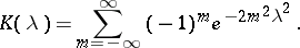 |
In 1948 N.V. Smirnov [BS] tabulated the Kolmogorov distribution function  . According to the Kolmogorov test with significance level
  ,
,  , the hypothesis
  must be rejected if
  , where
  is the critical value of the Kolmogorov test corresponding to the given significance level
  and is the root of the equation
  .
.
To determine  one recommends the use of the approximation of the limiting law of the Kolmogorov statistic
  and its limiting distribution; see [B], where it is shown that, as
  and
and  ,
,
 | (*) |
 |
The application of the approximation (*) gives the following approximation of the critical value:
 |
where  is the root of the equation
  .
.
In practice, for the calculation of the value of the statistic  one uses the fact that
 |
where
 |
 |
and  is the variational series (or set of order statistics) constructed from the sample
  . The Kolmogorov test has the following geometric interpretation (see Fig.).
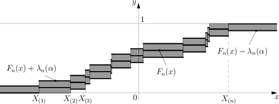
The graph of the functions  ,
,  is depicted in the
  -plane. The shaded region is the confidence zone at level
  for the distribution function
  , since if the hypothesis
  is true, then according to Kolmogorov's theorem
 |
If the graph of  does not leave the shaded region then, according to the Kolmogorov test,
  must be accepted with significance level
  ; otherwise
  is rejected.
The Kolmogorov test gave a strong impetus to the development of mathematical statistics, being the start of much research on new methods of statistical analysis lying at the foundations of non-parametric statistics.
References
| [K] | A.N. Kolmogorov, "Sulla determinizione empirica di una legge di distribuzione" Giorn. Ist. Ital. Attuari , 4 (1933) pp. 83–91 |
| [S] | N.V. Smirnov, "On estimating the discrepancy between empirical distribiution curves for two independent samples" Byull. Moskov. Gos. Univ. Ser. A , 2 : 2 (1938) pp. 3–14 (In Russian) |
| [B] | L.N. Bol'shev, "Asymptotically Pearson transformations" Theor. Probab. Appl. , 8 (1963) pp. 121–146 Teor. Veroyatnost. i Primenen. , 8 : 2 (1963) pp. 129–155 Zbl 0125.09103 |
| [BS] | L.N. Bol'shev, N.V. Smirnov, "Tables of mathematical statistics" , Libr. math. tables , 46 , Nauka (1983) (In Russian) (Processed by L.S. Bark and E.S. Kedrova) Zbl 0529.62099 |
Comments
Tests based on  and
and  , and similar tests for a two-sample problem based on
  and
and  , where
  is the empirical distribution function for samples of size
  for a population with distribution function
  , are also called Kolmogorov–Smirnov tests, cf. also Kolmogorov–Smirnov test.
References
| [N] | G.E. Noether, "A brief survey of nonparametric statistics" R.V. Hogg (ed.) , Studies in statistics , Math. Assoc. Amer. (1978) pp. 3–65 Zbl 0413.62023 |
| [HW] | M. Hollander, D.A. Wolfe, "Nonparametric statistical methods" , Wiley (1973) MR0353556 Zbl 0277.62030 |
Kolmogorov test. Encyclopedia of Mathematics. URL: http://encyclopediaofmath.org/index.php?title=Kolmogorov_test&oldid=26541