Difference between revisions of "Advertising, mathematics of"
(Importing text file) |
m (AUTOMATIC EDIT (latexlist): Replaced 175 formulas out of 178 by TEX code with an average confidence of 2.0 and a minimal confidence of 2.0.) |
||
| Line 1: | Line 1: | ||
| + | <!--This article has been texified automatically. Since there was no Nroff source code for this article, | ||
| + | the semi-automatic procedure described at https://encyclopediaofmath.org/wiki/User:Maximilian_Janisch/latexlist | ||
| + | was used. | ||
| + | If the TeX and formula formatting is correct, please remove this message and the {{TEX|semi-auto}} category. | ||
| + | |||
| + | Out of 178 formulas, 175 were replaced by TEX code.--> | ||
| + | |||
| + | {{TEX|semi-auto}}{{TEX|partial}} | ||
Advertising is one of the most important promotional tools of marketing. Its main purpose is to enhance buyers' responses to the organization and its offerings by providing information and by supplying reasons for preferring a particular organization's offer. | Advertising is one of the most important promotional tools of marketing. Its main purpose is to enhance buyers' responses to the organization and its offerings by providing information and by supplying reasons for preferring a particular organization's offer. | ||
| Line 12: | Line 20: | ||
Models of the size and allocation of the advertising budget vary widely, but most are closely related to the following general form: | Models of the size and allocation of the advertising budget vary widely, but most are closely related to the following general form: | ||
| − | Find | + | Find $u _ { i } ( t )$, $B$, to |
Maximize | Maximize | ||
| − | + | \begin{equation} \tag{a1} Z = \end{equation} | |
| − | + | \begin{equation*} = \sum _ { i } \sum _ { j } \sum _ { t } S _ { i } ( t | \{ u _ { i } ( t ) \} , \{ C _ { i j } ( t ) \} ) m _ { i } - \sum _ { i } \sum _ { t } u _ { i } ( t ) \end{equation*} | |
Subject to | Subject to | ||
| − | + | \begin{equation*} \sum _ { i } \sum _ { t } u _ { i } ( t ) \leq B (\text{budget constraint}), \end{equation*} | |
| − | + | \begin{equation*} L _ { i } \leq \sum u _ { i } ( t ) \leq U _ { i } \text{(regional constraint)}, \end{equation*} | |
where | where | ||
| − | + | $S _ { i } ( t | \{ u _ { i } ( t ) \} , \{ C _ { i j } ( t ) \} )$ is the sales in area $i$ at time $t$ as function of current and historical brand and competitive advertising; | |
| − | + | $C _ { i j } ( t )$ is the competitive advertising for competitor $j$ in area $i$; | |
| − | + | $u _ { i } ( t )$ is the advertising level in area $i$ at time $t$; | |
| − | + | $m_{i}$ is the margin per unit sales in area $i$; | |
| − | + | $\{ u_i ( t ) \}$ is the entire advertising program; | |
| − | + | $U_i$, $L_i$ are the upper and lower regional constraints; | |
| − | + | $B$ is the budget. Some researchers have developed a priori models [[#References|[a15]]] designed to postulate a general structure. Examples of this approach are the models of H.L. Vidale and H.B. Wolfe [[#References|[a24]]], M. Nerlove and K.J. Arrow [[#References|[a19]]], J.D.C. Little [[#References|[a13]]], [[#References|[a14]]], H. Simon [[#References|[a22]]], A.K. Basu and R. Batra [[#References|[a4]]], F.S. Zufryden [[#References|[a25]]], and V. Mahajan and E. Muller [[#References|[a17]]]. An alternative econometric approach starts with a specific data base, usually a time series of sales and advertising. These models include those by F. Bass [[#References|[a2]]], Bass and D.G. Clarke [[#References|[a3]]], D.B. Montgomery and A.J. Silk [[#References|[a18]]], J.J. Lambin [[#References|[a12]]], A.G. Rao and P.B. Miller [[#References|[a20]]], and J.O. Eastlack and A.G. Rao [[#References|[a7]]]. [[#References|[a8]]] provides a review of the econometric issues in advertising/sales response modeling. | |
| − | Mahajan and Muller [[#References|[a17]]] develop a model of the first type, where their focus is on the optimal shape of | + | Mahajan and Muller [[#References|[a17]]] develop a model of the first type, where their focus is on the optimal shape of $u ( t )$. Specifically, they look at whether advertising programs should be steady or turned on and off (pulsed). They use the following notation: |
| − | + | $a = B / \overline { u } T$ is the proportion of time (out of time $T$) that the firm advertises at level $u$; | |
| − | + | $k$ is the number of times the firm switches from advertising at $u$ to zero; | |
| − | + | $B$ is the advertising budget. For an even policy, the level of spending is $a \overline{u} $; for the pulsing policies, either $u$ or $0$ is spent. In general, in a $k$-pulsing policy | |
| − | + | \begin{equation} \tag{a2} u = \left\{ \begin{array} { c c } { \overline { u } } & { \text { for } \frac { i T } { k } \leq t < ( i + a ) \frac { T } { k }; } \\ { } & { 0 \leq i \leq k - 1, } \\ { 0 } & { \text { for } ( i + a ) \frac { T } { k } \leq t \leq ( i + 1 ) \frac { T } { k }, } \\ { } & { \text { and for } \ t = T ; 0 \leq i \leq k - 1. } \end{array} \right. \end{equation} | |
To link advertising pulsing to awareness they use the following functional form: | To link advertising pulsing to awareness they use the following functional form: | ||
| − | + | \begin{equation} \tag{a3} \frac { d A } { d t } = f ( u ) ( 1 - A ) - b A, \end{equation} | |
where | where | ||
| − | + | $A$ is the fraction of market aware of the product at any point in time; | |
| − | + | $b$ is the decay or forgetting parameter. Here, $f ( u ) ( 1 - A )$ is the "learning effect" and $b A$ is the "forgetting effect" . | |
The authors show that using any pulsing policy, awareness is | The authors show that using any pulsing policy, awareness is | ||
| − | <table class="eq" style="width:100%;"> <tr><td | + | <table class="eq" style="width:100%;"> <tr><td style="width:94%;text-align:center;" valign="top"><img align="absmiddle" border="0" src="https://www.encyclopediaofmath.org/legacyimages/a/a120/a120160/a12016040.png"/></td> <td style="width:5%;text-align:right;" valign="top">(a4)</td></tr></table> |
where | where | ||
| − | + | \begin{equation} \tag{a5} x = f ( \overline { u } ). \end{equation} | |
| − | With this model, the authors show that if | + | With this model, the authors show that if $f ( u )$ is $s$-shaped, then it generally pays to pulse and that more frequent pulsing is better. If $f ( u )$ is concave, however, an even advertising policy is best. |
A different approach to linking advertising to awareness has been proposed by K. Jedidi, J. Eliashberg and W.S. DeSarbo [[#References|[a10]]]. They model the system dynamics as: | A different approach to linking advertising to awareness has been proposed by K. Jedidi, J. Eliashberg and W.S. DeSarbo [[#References|[a10]]]. They model the system dynamics as: | ||
| − | + | \begin{equation} \tag{a6} A ( t ) = [ f ( u ( t ) ) + \beta ( X ( t ) - X ( t - \tau ) ) ] [ N _ { 0 } - A ( t ) ], \end{equation} | |
| − | + | \begin{equation*} A ( t _ { 0 } ) = A _ { 0 } , \dot { X } ( t ) = [ N ( X ( t ) , A ( t ) , t ) - X ( t ) ] \operatorname { exp } ( - k P ( t ) ), \end{equation*} | |
| − | + | \begin{equation*} X ( t _ { 0 } ) = X _ { 0 }. \end{equation*} | |
| − | For a general income density function | + | For a general income density function $g ( W )$, |
| − | + | \begin{equation} \tag{a7} N ( X ( t ) , A ( t ) , t ) = A ( t ) \int _ { a ( X ( t ) ) F + b } ^ { \infty } g ( W ) d W. \end{equation} | |
| − | Here, | + | Here, $A ( t )$ denotes the cumulative number of aware consumers, $X ( t )$ the cumulative number of adopters, $N_ 0 $ the size of the population of interest, $N ( . )$ the market potential, $u ( t )$ the advertising, and $P ( t )$ the price. The above equations are next incorporated into a dynamic problem and several propositions characterizing the optimal advertising (e.g., monotonically decreasing over time) and pricing (monotonic versus non-monotonic) are derived. |
A.G. Rao and Miller [[#References|[a20]]] provide an example of the econometric approach, developing a model which combines data from multiple markets over time. Their individual market model is | A.G. Rao and Miller [[#References|[a20]]] provide an example of the econometric approach, developing a model which combines data from multiple markets over time. Their individual market model is | ||
| − | + | \begin{equation} \tag{a8} S _ { t } = c _ { 0 } + c _ { 1 } u _ { t } + c _ { 1 } \lambda u _ { t - 1 } + c _ { 1 } \lambda ^ { 2 } u _ { t - 2 } + \ldots + \mu _ { t }, \end{equation} | |
where | where | ||
| − | + | $S _ { t }$ is the market share at $t$; | |
| − | + | $u _ { t }$ is the advertising spending at $t$; | |
| − | + | $c_0$, $c_1$, $\lambda$ are constants ($\lambda < 1$); | |
| − | + | $\mu _ { t }$ is the random disturbance. This equation means that an incremental expenditure of one unit of advertising in a given period will yield $c_1$ share points that period, $c _ { 1 } \lambda$ in the following period, $c _ { 1 } \lambda ^ { 2 }$ the period after that, etc. | |
| − | By multiplying (a8) by | + | By multiplying (a8) by $\lambda$, lagging it one period, and then subtracting that equation from the original equation (a8), one obtains: |
| − | + | \begin{equation} \tag{a9} S _ { t } = c _ { 0 } ( 1 - \lambda ) + \lambda S _ { t - 1 } + c _ { 1 } u _ { t } + \mu _ { t } - \lambda \mu _ { t - 1 } . \end{equation} | |
| − | Note that the short-run effect of advertising here is | + | Note that the short-run effect of advertising here is $d S _ { t } / d u _ { t } = c _ { 1 }$, while the long-run effect is $c_1$ in the first period, plus $\lambda c _ { 1 } + \lambda ^ { 2 } c _ { 1 } + \ldots$ in subsequent periods, or |
| − | + | \begin{equation} \tag{a10} \frac { c _ { 1 } } { 1 - \lambda }. \end{equation} | |
Now, let | Now, let | ||
| − | + | $I$ be the industry sales per year in district; | |
| − | + | $P$ be the district population; | |
| − | + | $A V$ be the average rate of advertising during the period. Then with $k$ periods per year, a unit increase in advertising produces a share increase of $c_1 / ( 1 - \lambda )$. Thus, the sales increase of an additional unit in advertising is | |
| − | + | \begin{equation} \tag{a11} y _ { i } = \Delta \text { sales } = \left( \frac { c _ { 1 } } { 1 - \lambda } \right) \frac { I } { k } ( \text { in market } i ) \end{equation} | |
| − | at a per capita advertising rate of | + | at a per capita advertising rate of $A V i / P = x_i$. In other words, (a11) can be interpreted as the derivative of a general response curve at the per capita spending rate $A V / P$. These results can then be used across markets to specify the slope of a more general response curve, enabling an optimal allocation of advertising spending. |
==Message and copy decisions.== | ==Message and copy decisions.== | ||
| Line 124: | Line 132: | ||
===Copy testing and measures of copy effectiveness.=== | ===Copy testing and measures of copy effectiveness.=== | ||
| − | See [[#References|[a11]]] for a report on the development and testing of a new advertising copy program for AT&T long lines, the "cost of visit" campaign. The cost of the visit campaign was tested against AT&T's very successful "reach out" campaign using a panel of | + | See [[#References|[a11]]] for a report on the development and testing of a new advertising copy program for AT&T long lines, the "cost of visit" campaign. The cost of the visit campaign was tested against AT&T's very successful "reach out" campaign using a panel of $16,000$ households. Because there is no (necessary) delay between the time an advertisement is shown and when someone can make a call, and because AT&T automatically records the transaction, response to advertising in this setting can be read much more clearly than in other field environments. |
The experiment lasted for over two years and had three phases: | The experiment lasted for over two years and had three phases: | ||
| − | 1) pre-assessment ( | + | 1) pre-assessment ($5$ months); |
| − | 2) treatment period ( | + | 2) treatment period ($15$ months); and |
| − | 3) post-assessment ( | + | 3) post-assessment ($6$ months). |
During the pre-assessment phase, records of all households were tracked to establish a norm for their calling behaviour. In addition, all respondents received a questionnaire to determine whether the test and control groups were demographically balanced (they were). | During the pre-assessment phase, records of all households were tracked to establish a norm for their calling behaviour. In addition, all respondents received a questionnaire to determine whether the test and control groups were demographically balanced (they were). | ||
| Line 142: | Line 150: | ||
USDF is the usage difference between test group (cost of visit) and control group (reach-out); | USDF is the usage difference between test group (cost of visit) and control group (reach-out); | ||
| − | UNOFF is | + | UNOFF is $0$ for pre-test weeks and $1$ for test weeks; |
| − | <img align="absmiddle" border="0" src="https://www.encyclopediaofmath.org/legacyimages/a/a120/a120160/a12016089.png" /> is the disturbance. | + | <img align="absmiddle" border="0" src="https://www.encyclopediaofmath.org/legacyimages/a/a120/a120160/a12016089.png"/> is the disturbance. |
The equation | The equation | ||
| − | + | \begin{equation} \tag{a12} \operatorname{USDF} = \alpha + \beta \operatorname{UNOFF} + \epsilon \end{equation} | |
| − | models the difference in usage/household/week as a pre-period constant ( | + | models the difference in usage/household/week as a pre-period constant ($\alpha$) and a treatment constant ($\alpha + \beta$). So the statistical significance of $\beta$ for any segment (light users in a deep discount period, for example), can be read from standard confidence limits resulting from linear regression analysis. |
In order to project the results to the national level, they used the following model: | In order to project the results to the national level, they used the following model: | ||
| − | + | \begin{equation} \tag{a13} y = \sum _ { i = 1 } ^ { I } \left( n _ { i } \sum _ { j = 1 } ^ { J } z _ { i j } p _ { i j } \right), \end{equation} | |
where | where | ||
| − | + | $y$ is the projected usage in a given area, assuming a given level of advertising exposure; | |
| − | + | $i$ is the index of usage segment (light, regular, etc.), $i = 1 , \ldots , I$; | |
| − | + | $j$ is the index of calling category (rate period), $j = 1 , \ldots , J$; | |
| − | + | $z_{i j }$ is the usage measure per households in cell $i$ for calling category $j$; | |
| − | + | $n_i$ is the number of households of segment type $i$ in the area; | |
| − | + | $p _ { ij }$ is the fraction increase or decrease in cell $i$, category $j$ for "cost of visit" versus "reach-out" . | |
The national or any regional projection can be made by summing over the appropriate areas. | The national or any regional projection can be made by summing over the appropriate areas. | ||
| Line 175: | Line 183: | ||
===Estimating the creative quality of advertisements.=== | ===Estimating the creative quality of advertisements.=== | ||
| − | In a study of the effectiveness of industrial print advertisements, D.M. Hanssens and B.A. Weitz [[#References|[a9]]] related | + | In a study of the effectiveness of industrial print advertisements, D.M. Hanssens and B.A. Weitz [[#References|[a9]]] related $24$ ad characteristics to recall, readership, and inquiry generation for $1,160$ industrial advertisements in Electronic Design. They used a model of the form |
| − | + | \begin{equation} \tag{a14} y _ { i } = e ^ { a} \prod _ { j = 1 } ^ { p _ { t } } x _ { i j } ^ { b j } \prod _ { j ^ { \prime } = p _ { t + 1 } } ^ { p } ( 1 + x _ { i j ^ { \prime } } ) ^ { b j ^ { \prime } } e ^ { \mu i }, \end{equation} | |
where | where | ||
| − | + | $y _ { i }$ is the effectiveness measure for the $i$th advertisement; | |
| − | + | $x _ { ij }$ is the value of the $j$th non-binary characteristic of the $i$th advertisement (page number, advertisement size), $j = 1 , \ldots , p _ { t }$; | |
| − | + | $x _ { i j^{\prime} }$ is the value ($0$ or $1$) of the $j ^ { \prime }$th binary characteristic of the $i$th advertisement (bleed, colour, etc.), $j ^ { \prime } = p _ { t + 1} , \ldots , p$; | |
| − | + | $e ^ { a }$ is the scale factor; | |
| − | + | $\mu _ { i }$ is the error term. They segmented $15$ product groups into three categories (routine purchase items, unique purchase items, and important purchase items) by factor analysis of purchasing-process similarity ratings obtained from readers of the magazine. They found that advertising characteristics accounted for more than 45% of the variance in the "seen" effectiveness measure, more than 30% of the read-most effectiveness measure, and between 19% and 36% of the variance in inquiry generation. | |
They also found that recall and readership were strongly related to format and layout variables (advertisement size, colours, bleed, use of photographs/illustrations, etc.), while the effects were weaker for inquiry generation. The effects of some factors, such as advertisement size, were consistently related across product groups and effectiveness measures, while others, such as the use of attention-getting methods (woman in advertisements, size of headline, etc.) were specific to the product category and the effectiveness measure. | They also found that recall and readership were strongly related to format and layout variables (advertisement size, colours, bleed, use of photographs/illustrations, etc.), while the effects were weaker for inquiry generation. The effects of some factors, such as advertisement size, were consistently related across product groups and effectiveness measures, while others, such as the use of attention-getting methods (woman in advertisements, size of headline, etc.) were specific to the product category and the effectiveness measure. | ||
| Line 215: | Line 223: | ||
The effect of exposures on audience awareness depends on the exposures' reach, frequency, and impact: | The effect of exposures on audience awareness depends on the exposures' reach, frequency, and impact: | ||
| − | Reach ( | + | Reach ($R$): The number of different persons or households exposed to a particular media schedule at least once during the specified time period; |
| − | Frequency ( | + | Frequency ($F$): The number of times within a specified time period that an average person or household is exposed to the message; |
| − | Impact ( | + | Impact ($I$): The qualitative value of an exposure through a given medium (thus, a food advertisement would have a higher impact in good housekeeping than it would have in popular mechanics). |
| − | The weighted number of exposures ( | + | The weighted number of exposures ($W E$) is the reach times the average frequency times the average impact, that is, |
| − | + | \begin{equation} \tag{a15} W E = R.F.I. \end{equation} | |
The media-planning problem can now be viewed as follows. With a given budget, what is the most cost-effective combination of reach, frequency, and impact to buy? | The media-planning problem can now be viewed as follows. With a given budget, what is the most cost-effective combination of reach, frequency, and impact to buy? | ||
| Line 233: | Line 241: | ||
the level of audience duplication across all pairs of vehicles. In the case of two media alternatives one would typically have an equation for net coverage as follows: | the level of audience duplication across all pairs of vehicles. In the case of two media alternatives one would typically have an equation for net coverage as follows: | ||
| − | + | \begin{equation} \tag{a16} R = r _ { 1 } ( X _ { 1 } ) + r _ { 2 } ( X _ { 2 } ) - r _ { 12 } ( X _ { 12 } ), \end{equation} | |
where | where | ||
| − | + | $R$ is the reach of the media schedule (i.e., total weighted-exposure value with replication and duplication removed); | |
| − | + | $r _ { i } ( X _ { i } )$ is the number of persons in the audience of media $i$; | |
| − | + | $r _ { 12 } ( X _ { 12 } )$ is the number of persons in the audience of both media vehicles. (The $r _ { i } ( X _ { i } )$ are typically concave; an old study of the "Saturday Evening Post" showed only 55% more families are reached with $13$ issues than with $1$ issue.) Equation (a16) can be easily generalized to the case of $n$ media alternatives. | |
| − | Modeling approaches to media scheduling have relied heavily on [[Mathematical programming|mathematical programming]] procedures. MEDIAC [[#References|[a16]]], for instance, assumes an advertiser is seeking to buy media for a year with | + | Modeling approaches to media scheduling have relied heavily on [[Mathematical programming|mathematical programming]] procedures. MEDIAC [[#References|[a16]]], for instance, assumes an advertiser is seeking to buy media for a year with $B$ dollars that will maximize sales. He or she can identify $S$ different segments of the market, and for each segment $i$ (s)he can estimate its sales potential in time period $t$: |
| − | + | \begin{equation} \tag{a17} \overline { Q _ { it } } = n _ { i } q _ { it }, \end{equation} | |
where | where | ||
| − | + | $Q_{it}$ is the sales potential of market segment $i$ in time period $t$ (potential units per time period); | |
| − | + | $n_i$ is the number of people in market segment $i$; | |
| − | + | $q_{ it}$ is the sales potential of person in segment $i$ in period $t$ (potential units per capita per time period). | |
| − | The sales potential represents the maximum attainable sales in a segment in a given time period. The more dollars spent on advertising in media reaching that segment, the higher the per capita exposure level and the higher the percentage-of-sales potential that will be realized. Thus, the percentage-of-sales potential realized is a function of the per capita exposure level, | + | The sales potential represents the maximum attainable sales in a segment in a given time period. The more dollars spent on advertising in media reaching that segment, the higher the per capita exposure level and the higher the percentage-of-sales potential that will be realized. Thus, the percentage-of-sales potential realized is a function of the per capita exposure level, $f ( y_{i t} )$, where |
| − | + | $y_{it}$ is the exposure level of an average individual in market segment $i$ in time period $t$ (exposure value per capita). The problem of finding the best media plan can be stated as trying to: | |
| − | Find the | + | Find the $x _ { j t }$ for all $j$ and $t$ that will |
Maximize | Maximize | ||
| − | + | \begin{equation} \tag{a18} \sum _ { i = 1 } ^ { S } \sum _ { t = 1 } ^ { T } n _ { t } q _ { i t } f ( y _ { i t } ) \end{equation} | |
Subject to: | Subject to: | ||
| Line 269: | Line 277: | ||
current exposure-value constraints | current exposure-value constraints | ||
| − | + | \begin{equation} \tag{a19} y _ { i t } = \alpha y _ { i , t - 1 } + \sum _ { j = 1 } ^ { N } k _ { i j t } e _ { i j } x _ { j t }; \end{equation} | |
lower and upper media-use rate constraints, where | lower and upper media-use rate constraints, where | ||
| − | + | \begin{equation} \tag{a20} l _ { j t } \leq x _ { j t } \leq u _ { j t }; \end{equation} | |
a budget constraint | a budget constraint | ||
| − | + | \begin{equation} \tag{a21} \sum _ { j = 1 } ^ { N } \sum _ { t = 1 } ^ { T } c _ { j t } x _ { j t } \leq B, \end{equation} | |
where | where | ||
| − | + | $e_{ij}$ is the exposure value of one exposure in media vehicle $j$ to a person in market segment $i$; | |
| − | + | $k_{i j t}$ is the expected number of exposures produced in market segment $i$ by one insertion in media vehicle $j$ in time period $t$; | |
| − | + | $x _ { j t }$ is the number of exposures in media vehicle $j$ in time period $t$; | |
| − | + | $\alpha$ is the carry-over effect ($\alpha \in ( 0,1 )$), the amount of exposure in period $t$ in the absence of new advertising that period; | |
and non-negativity constraints | and non-negativity constraints | ||
| − | + | \begin{equation} \tag{a22} x _ { j t } , y _ { i t } \geq 0. \end{equation} | |
| − | In this form, the problem has a non-linear but separable objective function that is subject to linear constraints. If the non-linear objective function is concave, the problem can be solved by piecewise-linear approximation techniques. If it is | + | In this form, the problem has a non-linear but separable objective function that is subject to linear constraints. If the non-linear objective function is concave, the problem can be solved by piecewise-linear approximation techniques. If it is $s$-shaped and the problem is of modest size, it can be solved by [[Dynamic programming|dynamic programming]] [[#References|[a16]]]. If the problem is not of modest size, [[#References|[a16]]] shows that satisfactory, though not necessarily optimal solutions can be obtained through the use of heuristic methods. |
MEDIAC represents an important attempt to include the dimensions of market segments, sales potentials, diminishing marginal returns, forgetting, and timing into a media-planning model. Other heuristic procedures include those in [[#References|[a21]]], [[#References|[a23]]], the Solem model [[#References|[a5]]], and the ADMOD model [[#References|[a1]]]. | MEDIAC represents an important attempt to include the dimensions of market segments, sales potentials, diminishing marginal returns, forgetting, and timing into a media-planning model. Other heuristic procedures include those in [[#References|[a21]]], [[#References|[a23]]], the Solem model [[#References|[a5]]], and the ADMOD model [[#References|[a1]]]. | ||
| Line 303: | Line 311: | ||
====References==== | ====References==== | ||
| − | <table>< | + | <table><tr><td valign="top">[a1]</td> <td valign="top"> D.A. Aaker, "Admod: An advertising decision model" ''J. Marketing Research'' , '''12''' : February (1975) pp. 37–45</td></tr><tr><td valign="top">[a2]</td> <td valign="top"> F. Bass, "A simultaneous equation regression study of advertising and sales of cigarettes" ''J. Marketing Research'' , '''6''' (1969) pp. 291–300</td></tr><tr><td valign="top">[a3]</td> <td valign="top"> F. Bass, D.G. Clarke, "Testing distributed lag models of advertising effects" ''J. Marketing Research'' , '''9''' (1972) pp. 298–308</td></tr><tr><td valign="top">[a4]</td> <td valign="top"> A.K. Basu, R. Batra, "Ad Split: A multi-brand advertising budget allocation model" ''J. Advertising'' , '''17''' (1988) pp. 44–51</td></tr><tr><td valign="top">[a5]</td> <td valign="top"> E.B. Bimm, A.G. Millman, "A model for planning TV in canada" ''J. Advertising Research'' , '''18''' : 4 (1978) pp. 43–48</td></tr><tr><td valign="top">[a6]</td> <td valign="top"> R.R. Burke, A. Rangaswamy, J. Wind, J. Eliashberg, "A knowledge-based system for advertising design" ''Marketing Science'' , '''9''' : 3 (1990) pp. 212–229</td></tr><tr><td valign="top">[a7]</td> <td valign="top"> J.O. Eastlack, A.G. Rao, "Modeling response to advertising and price changes for 'V-8' cocktail vegetable juice" ''Marketing Science'' , '''5''' : 3 (1986) pp. 245–259</td></tr><tr><td valign="top">[a8]</td> <td valign="top"> D.M. Hanssens, L.J. Parsons, R.L. Schultz, "Market response models: Econometric and time series analysis" , Kluwer Acad. Publ. (1990)</td></tr><tr><td valign="top">[a9]</td> <td valign="top"> D.M. Hanssens, B.A. Weitz, "The effectiveness of industrial print advertisements across product categories" ''J. Marketing Research'' , '''17''' : August (1980) pp. 294–306</td></tr><tr><td valign="top">[a10]</td> <td valign="top"> K. Jedidi, J. Eliashberg, W.S. DeSarbo, "Optimal advertising and pricing for a three-stage time-lagged monopolistic diffusion model incorporating income" ''Optimal Control Appl. Methods'' , '''10''' : October – December (1989) pp. 313–331</td></tr><tr><td valign="top">[a11]</td> <td valign="top"> A.P. Kuritsky, J.D.C. Little, A.J. Silk, E.S. Bassman, "The development, testing and execution of a new marketing strategy at AT&T long lives" ''Interfaces'' , '''12''' : 6 (December) (1982) pp. 22–37</td></tr><tr><td valign="top">[a12]</td> <td valign="top"> J.J. Lambin, "Advertising, competition and market conduct in oligopoly over time" , North-Holland (1976)</td></tr><tr><td valign="top">[a13]</td> <td valign="top"> J.D.C. Little, "A model of adaptive control of promotional spending" ''Oper. Res.'' , '''14''' (1966) pp. 1075–1097</td></tr><tr><td valign="top">[a14]</td> <td valign="top"> J.D.C. Little, "Brandaid: A marketing mix model; Part I: Structure; Part II: Implementation" ''Oper. Res.'' , '''23''' (1975) pp. 628–673</td></tr><tr><td valign="top">[a15]</td> <td valign="top"> J.D.C. Little, "Aggregate advertising models: The state of the art" ''Oper. Res.'' , '''27''' : 4 (July/August) (1979) pp. 629–667</td></tr><tr><td valign="top">[a16]</td> <td valign="top"> J.D.C. Little, L.M. Lodish, "A media planning calculus" ''Oper. Res.'' , '''17''' : January/February (1969) pp. 1–35</td></tr><tr><td valign="top">[a17]</td> <td valign="top"> V. Mahajan, E. Muller, "Advertising pulsing policies for generating awareness for new products" ''Marketing Science'' , '''5''' : 2 (Spring) (1986) pp. 86–106</td></tr><tr><td valign="top">[a18]</td> <td valign="top"> D.B. Montgomery, A.J. Silk, "Estimating dynamic effects of marketing communications expenditures" ''Management Science'' , '''18''' : June (1972) pp. B485–B501</td></tr><tr><td valign="top">[a19]</td> <td valign="top"> M. Nerlove, K.J. Arrow, "Optimal advertising policy under dynamic conditions" ''Econometrica'' , '''29''' : May (1962) pp. 129–142</td></tr><tr><td valign="top">[a20]</td> <td valign="top"> A.G. Rao, P.B. Miller, "Advertising/sales response functions" ''J. Advertising Research'' , '''15''' (1975) pp. 7–15</td></tr><tr><td valign="top">[a21]</td> <td valign="top"> R.T. Rust, N. Eechambadi, "Scheduling network television programs: A heuristic audience flow approach to maximize audience share" ''J. Advertising'' , '''18''' : 2 (1989) pp. 11–18</td></tr><tr><td valign="top">[a22]</td> <td valign="top"> H. Simon, "Adpuls: An advertising model with wearout and pulsation" ''J. Marketing Research'' , '''19''' : August (1982) pp. 352–363</td></tr><tr><td valign="top">[a23]</td> <td valign="top"> G.L. Urban, "National and local allocation of advertising dollars" ''J. Marketing Research'' , '''15''' : 6 (1975) pp. 7–16</td></tr><tr><td valign="top">[a24]</td> <td valign="top"> H.L. Vidale, H.B. Wolfe, "An operations research study of sales response to advertising" ''Oper. Res.'' , '''5''' (1957) pp. 370–381</td></tr><tr><td valign="top">[a25]</td> <td valign="top"> F.S. Zufryden, "How much should be spent for advertising a brand?" ''J. Advertising Research'' , '''29''' : 2 (April/May) (1989) pp. 24–34</td></tr></table> |
Revision as of 16:57, 1 July 2020
Advertising is one of the most important promotional tools of marketing. Its main purpose is to enhance buyers' responses to the organization and its offerings by providing information and by supplying reasons for preferring a particular organization's offer.
Advertising decisions address an interrelated set of issues, including:
a) how much to spend in total and in the allocation of that budget;
b) how to determine the best messages to deliver with advertising; and
c) what media schedule delivers these messages to the target audience best. Although these decisions clearly interact (for example, a more effective advertising message may permit a lower total advertising budget), researchers have traditionally modeled these phenomena separately.
Advertising budget setting and allocation.
Models of the size and allocation of the advertising budget vary widely, but most are closely related to the following general form:
Find $u _ { i } ( t )$, $B$, to
Maximize
\begin{equation} \tag{a1} Z = \end{equation}
\begin{equation*} = \sum _ { i } \sum _ { j } \sum _ { t } S _ { i } ( t | \{ u _ { i } ( t ) \} , \{ C _ { i j } ( t ) \} ) m _ { i } - \sum _ { i } \sum _ { t } u _ { i } ( t ) \end{equation*}
Subject to
\begin{equation*} \sum _ { i } \sum _ { t } u _ { i } ( t ) \leq B (\text{budget constraint}), \end{equation*}
\begin{equation*} L _ { i } \leq \sum u _ { i } ( t ) \leq U _ { i } \text{(regional constraint)}, \end{equation*}
where
$S _ { i } ( t | \{ u _ { i } ( t ) \} , \{ C _ { i j } ( t ) \} )$ is the sales in area $i$ at time $t$ as function of current and historical brand and competitive advertising;
$C _ { i j } ( t )$ is the competitive advertising for competitor $j$ in area $i$;
$u _ { i } ( t )$ is the advertising level in area $i$ at time $t$;
$m_{i}$ is the margin per unit sales in area $i$;
$\{ u_i ( t ) \}$ is the entire advertising program;
$U_i$, $L_i$ are the upper and lower regional constraints;
$B$ is the budget. Some researchers have developed a priori models [a15] designed to postulate a general structure. Examples of this approach are the models of H.L. Vidale and H.B. Wolfe [a24], M. Nerlove and K.J. Arrow [a19], J.D.C. Little [a13], [a14], H. Simon [a22], A.K. Basu and R. Batra [a4], F.S. Zufryden [a25], and V. Mahajan and E. Muller [a17]. An alternative econometric approach starts with a specific data base, usually a time series of sales and advertising. These models include those by F. Bass [a2], Bass and D.G. Clarke [a3], D.B. Montgomery and A.J. Silk [a18], J.J. Lambin [a12], A.G. Rao and P.B. Miller [a20], and J.O. Eastlack and A.G. Rao [a7]. [a8] provides a review of the econometric issues in advertising/sales response modeling.
Mahajan and Muller [a17] develop a model of the first type, where their focus is on the optimal shape of $u ( t )$. Specifically, they look at whether advertising programs should be steady or turned on and off (pulsed). They use the following notation:
$a = B / \overline { u } T$ is the proportion of time (out of time $T$) that the firm advertises at level $u$;
$k$ is the number of times the firm switches from advertising at $u$ to zero;
$B$ is the advertising budget. For an even policy, the level of spending is $a \overline{u} $; for the pulsing policies, either $u$ or $0$ is spent. In general, in a $k$-pulsing policy
\begin{equation} \tag{a2} u = \left\{ \begin{array} { c c } { \overline { u } } & { \text { for } \frac { i T } { k } \leq t < ( i + a ) \frac { T } { k }; } \\ { } & { 0 \leq i \leq k - 1, } \\ { 0 } & { \text { for } ( i + a ) \frac { T } { k } \leq t \leq ( i + 1 ) \frac { T } { k }, } \\ { } & { \text { and for } \ t = T ; 0 \leq i \leq k - 1. } \end{array} \right. \end{equation}
To link advertising pulsing to awareness they use the following functional form:
\begin{equation} \tag{a3} \frac { d A } { d t } = f ( u ) ( 1 - A ) - b A, \end{equation}
where
$A$ is the fraction of market aware of the product at any point in time;
$b$ is the decay or forgetting parameter. Here, $f ( u ) ( 1 - A )$ is the "learning effect" and $b A$ is the "forgetting effect" .
The authors show that using any pulsing policy, awareness is
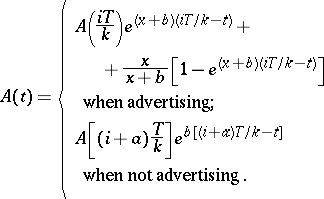 | (a4) |
where
\begin{equation} \tag{a5} x = f ( \overline { u } ). \end{equation}
With this model, the authors show that if $f ( u )$ is $s$-shaped, then it generally pays to pulse and that more frequent pulsing is better. If $f ( u )$ is concave, however, an even advertising policy is best.
A different approach to linking advertising to awareness has been proposed by K. Jedidi, J. Eliashberg and W.S. DeSarbo [a10]. They model the system dynamics as:
\begin{equation} \tag{a6} A ( t ) = [ f ( u ( t ) ) + \beta ( X ( t ) - X ( t - \tau ) ) ] [ N _ { 0 } - A ( t ) ], \end{equation}
\begin{equation*} A ( t _ { 0 } ) = A _ { 0 } , \dot { X } ( t ) = [ N ( X ( t ) , A ( t ) , t ) - X ( t ) ] \operatorname { exp } ( - k P ( t ) ), \end{equation*}
\begin{equation*} X ( t _ { 0 } ) = X _ { 0 }. \end{equation*}
For a general income density function $g ( W )$,
\begin{equation} \tag{a7} N ( X ( t ) , A ( t ) , t ) = A ( t ) \int _ { a ( X ( t ) ) F + b } ^ { \infty } g ( W ) d W. \end{equation}
Here, $A ( t )$ denotes the cumulative number of aware consumers, $X ( t )$ the cumulative number of adopters, $N_ 0 $ the size of the population of interest, $N ( . )$ the market potential, $u ( t )$ the advertising, and $P ( t )$ the price. The above equations are next incorporated into a dynamic problem and several propositions characterizing the optimal advertising (e.g., monotonically decreasing over time) and pricing (monotonic versus non-monotonic) are derived.
A.G. Rao and Miller [a20] provide an example of the econometric approach, developing a model which combines data from multiple markets over time. Their individual market model is
\begin{equation} \tag{a8} S _ { t } = c _ { 0 } + c _ { 1 } u _ { t } + c _ { 1 } \lambda u _ { t - 1 } + c _ { 1 } \lambda ^ { 2 } u _ { t - 2 } + \ldots + \mu _ { t }, \end{equation}
where
$S _ { t }$ is the market share at $t$;
$u _ { t }$ is the advertising spending at $t$;
$c_0$, $c_1$, $\lambda$ are constants ($\lambda < 1$);
$\mu _ { t }$ is the random disturbance. This equation means that an incremental expenditure of one unit of advertising in a given period will yield $c_1$ share points that period, $c _ { 1 } \lambda$ in the following period, $c _ { 1 } \lambda ^ { 2 }$ the period after that, etc.
By multiplying (a8) by $\lambda$, lagging it one period, and then subtracting that equation from the original equation (a8), one obtains:
\begin{equation} \tag{a9} S _ { t } = c _ { 0 } ( 1 - \lambda ) + \lambda S _ { t - 1 } + c _ { 1 } u _ { t } + \mu _ { t } - \lambda \mu _ { t - 1 } . \end{equation}
Note that the short-run effect of advertising here is $d S _ { t } / d u _ { t } = c _ { 1 }$, while the long-run effect is $c_1$ in the first period, plus $\lambda c _ { 1 } + \lambda ^ { 2 } c _ { 1 } + \ldots$ in subsequent periods, or
\begin{equation} \tag{a10} \frac { c _ { 1 } } { 1 - \lambda }. \end{equation}
Now, let
$I$ be the industry sales per year in district;
$P$ be the district population;
$A V$ be the average rate of advertising during the period. Then with $k$ periods per year, a unit increase in advertising produces a share increase of $c_1 / ( 1 - \lambda )$. Thus, the sales increase of an additional unit in advertising is
\begin{equation} \tag{a11} y _ { i } = \Delta \text { sales } = \left( \frac { c _ { 1 } } { 1 - \lambda } \right) \frac { I } { k } ( \text { in market } i ) \end{equation}
at a per capita advertising rate of $A V i / P = x_i$. In other words, (a11) can be interpreted as the derivative of a general response curve at the per capita spending rate $A V / P$. These results can then be used across markets to specify the slope of a more general response curve, enabling an optimal allocation of advertising spending.
Message and copy decisions.
Much of the effect of an advertising exposure depends on the creative quality of the advertising itself. But rating the quality of the advertising is difficult: an advertisement may have good aesthetic properties and win awards, and yet it may not do much for sales. Another advertisement may seem crude and offensive, and yet it may be a major force behind sales.
Copy testing and measures of copy effectiveness.
See [a11] for a report on the development and testing of a new advertising copy program for AT&T long lines, the "cost of visit" campaign. The cost of the visit campaign was tested against AT&T's very successful "reach out" campaign using a panel of $16,000$ households. Because there is no (necessary) delay between the time an advertisement is shown and when someone can make a call, and because AT&T automatically records the transaction, response to advertising in this setting can be read much more clearly than in other field environments.
The experiment lasted for over two years and had three phases:
1) pre-assessment ($5$ months);
2) treatment period ($15$ months); and
3) post-assessment ($6$ months).
During the pre-assessment phase, records of all households were tracked to establish a norm for their calling behaviour. In addition, all respondents received a questionnaire to determine whether the test and control groups were demographically balanced (they were).
During the treatment period the two advertising campaigns were aired at a rate that gave each household about three exposures per week. The objective of the "cost of visit" campaign was to encourage all user groups, but particularly the light user group, to call during the 60%-off deep discount period (nights and weekends). In the experiment, there was an overall increase in revenue of about 1% overall with the targeted light user group yielding a 15% increase in revenue.
In order to make these assessments and to project them to the national level, they used the following definitions:
USDF is the usage difference between test group (cost of visit) and control group (reach-out);
UNOFF is $0$ for pre-test weeks and $1$ for test weeks;
 is the disturbance.
The equation
\begin{equation} \tag{a12} \operatorname{USDF} = \alpha + \beta \operatorname{UNOFF} + \epsilon \end{equation}
models the difference in usage/household/week as a pre-period constant ($\alpha$) and a treatment constant ($\alpha + \beta$). So the statistical significance of $\beta$ for any segment (light users in a deep discount period, for example), can be read from standard confidence limits resulting from linear regression analysis.
In order to project the results to the national level, they used the following model:
\begin{equation} \tag{a13} y = \sum _ { i = 1 } ^ { I } \left( n _ { i } \sum _ { j = 1 } ^ { J } z _ { i j } p _ { i j } \right), \end{equation}
where
$y$ is the projected usage in a given area, assuming a given level of advertising exposure;
$i$ is the index of usage segment (light, regular, etc.), $i = 1 , \ldots , I$;
$j$ is the index of calling category (rate period), $j = 1 , \ldots , J$;
$z_{i j }$ is the usage measure per households in cell $i$ for calling category $j$;
$n_i$ is the number of households of segment type $i$ in the area;
$p _ { ij }$ is the fraction increase or decrease in cell $i$, category $j$ for "cost of visit" versus "reach-out" .
The national or any regional projection can be made by summing over the appropriate areas.
The results of the analysis showed that AT&T could expect to earn more than $100 million more from the segment they targeted without any increase in capital expenditures by introducing this new ad copy. ==='"`UNIQ--h-3--QINU`"'Estimating the creative quality of advertisements.=== In a study of the effectiveness of industrial print advertisements, D.M. Hanssens and B.A. Weitz [[#References|[a9]]] related $24$ ad characteristics to recall, readership, and inquiry generation for $1,160$ industrial advertisements in Electronic Design. They used a model of the form \begin{equation} \tag{a14} y _ { i } = e ^ { a} \prod _ { j = 1 } ^ { p _ { t } } x _ { i j } ^ { b j } \prod _ { j ^ { \prime } = p _ { t + 1 } } ^ { p } ( 1 + x _ { i j ^ { \prime } } ) ^ { b j ^ { \prime } } e ^ { \mu i }, \end{equation} where $y _ { i }$ is the effectiveness measure for the $i$th advertisement; $x _ { ij }$ is the value of the $j$th non-binary characteristic of the $i$th advertisement (page number, advertisement size), $j = 1 , \ldots , p _ { t }$; $x _ { i j^{\prime} }$ is the value ($0$ or $1$) of the $j ^ { \prime }$th binary characteristic of the $i$th advertisement (bleed, colour, etc.), $j ^ { \prime } = p _ { t + 1} , \ldots , p$; $e ^ { a }$ is the scale factor; $\mu _ { i }$ is the error term. They segmented $15$ product groups into three categories (routine purchase items, unique purchase items, and important purchase items) by factor analysis of purchasing-process similarity ratings obtained from readers of the magazine. They found that advertising characteristics accounted for more than 45% of the variance in the "seen" effectiveness measure, more than 30% of the read-most effectiveness measure, and between 19% and 36% of the variance in inquiry generation. They also found that recall and readership were strongly related to format and layout variables (advertisement size, colours, bleed, use of photographs/illustrations, etc.), while the effects were weaker for inquiry generation. The effects of some factors, such as advertisement size, were consistently related across product groups and effectiveness measures, while others, such as the use of attention-getting methods (woman in advertisements, size of headline, etc.) were specific to the product category and the effectiveness measure. ==='"`UNIQ--h-4--QINU`"'Advertising copy design.=== Advertising copy design is usually viewed as a non-quantitative, creative process. R.R. Burke, A. Rangsaswamy, Eliashberg, and J. Wind [[#References|[a6]]] developed a rule-based system for advertisement copy design, demonstrating that this view is not altogether true. ADCAD is a rule-based expert system that allows managers to translate their qualitative perception of marketplace behaviour into a basis for deciding on advertising design. The ADCAD system assumes that before purchasing a brand a consumer must 1) have a need that can be satisfied by purchasing this brand; 2) be aware that the brand can satisfy this need; 3) recognize the brand and distinguish it from its close substitutes; and 4) have no other behavioural or attitudinal obstacles to purchasing the brand. Advertising can address one or more of these issues: it can stimulate demand for the product category, create brand awareness, facilitate brand recognition, and modify beliefs about the brand that might be barriers to purchase. ADCAD starts by asking for background information about the product, the nature of competition, the characteristics of the target audience(s), etc., and it then develops a communication strategy for each target audience. Using knowledge base from experts and the published literature, based on artificial intelligence inference engine, ADCAD then selects communications approaches to achieve the advertising and marketing objectives consistent with the characteristics of the consumers, the product, and the environment. It makes recommendations concerning the position of the advertisement, the characteristics of the message, the characteristics of the presenter, and the emotional tone of the advertisement. While ADCAD does not exhibit the creative potential of human copywriters, it does provide important input into the development and assessment of advertising copy. =='"`UNIQ--h-5--QINU`"'Media selection and scheduling.== Media selection addresses how to find the best way to deliver the desired number of exposures to the target audience and to schedule the delivery of those exposures over the planning period. The effect of exposures on audience awareness depends on the exposures' reach, frequency, and impact: Reach ($R$): The number of different persons or households exposed to a particular media schedule at least once during the specified time period; Frequency ($F$): The number of times within a specified time period that an average person or household is exposed to the message; Impact ($I$): The qualitative value of an exposure through a given medium (thus, a food advertisement would have a higher impact in good housekeeping than it would have in popular mechanics). The weighted number of exposures ($W E$) is the reach times the average frequency times the average impact, that is, \begin{equation} \tag{a15} W E = R.F.I. \end{equation} The media-planning problem can now be viewed as follows. With a given budget, what is the most cost-effective combination of reach, frequency, and impact to buy? To determine the total weighted-exposure value of a media schedule, one must know two things: the net cumulative audience of each media vehicle as a function of the number of exposures; and the level of audience duplication across all pairs of vehicles. In the case of two media alternatives one would typically have an equation for net coverage as follows: \begin{equation} \tag{a16} R = r _ { 1 } ( X _ { 1 } ) + r _ { 2 } ( X _ { 2 } ) - r _ { 12 } ( X _ { 12 } ), \end{equation} where $R$ is the reach of the media schedule (i.e., total weighted-exposure value with replication and duplication removed); $r _ { i } ( X _ { i } )$ is the number of persons in the audience of media $i$; $r _ { 12 } ( X _ { 12 } )$ is the number of persons in the audience of both media vehicles. (The $r _ { i } ( X _ { i } )$ are typically concave; an old study of the "Saturday Evening Post" showed only 55% more families are reached with $13$ issues than with $1$ issue.) Equation (a16) can be easily generalized to the case of $n$ media alternatives. Modeling approaches to media scheduling have relied heavily on [[Mathematical programming|mathematical programming]] procedures. MEDIAC [[#References|[a16]]], for instance, assumes an advertiser is seeking to buy media for a year with $B$ dollars that will maximize sales. He or she can identify $S$ different segments of the market, and for each segment $i$ (s)he can estimate its sales potential in time period $t$: \begin{equation} \tag{a17} \overline { Q _ { it } } = n _ { i } q _ { it }, \end{equation} where $Q_{it}$ is the sales potential of market segment $i$ in time period $t$ (potential units per time period); $n_i$ is the number of people in market segment $i$; $q_{ it}$ is the sales potential of person in segment $i$ in period $t$ (potential units per capita per time period). The sales potential represents the maximum attainable sales in a segment in a given time period. The more dollars spent on advertising in media reaching that segment, the higher the per capita exposure level and the higher the percentage-of-sales potential that will be realized. Thus, the percentage-of-sales potential realized is a function of the per capita exposure level, $f ( y_{i t} )$, where $y_{it}$ is the exposure level of an average individual in market segment $i$ in time period $t$ (exposure value per capita). The problem of finding the best media plan can be stated as trying to: Find the $x _ { j t }$ for all $j$ and $t$ that will Maximize \begin{equation} \tag{a18} \sum _ { i = 1 } ^ { S } \sum _ { t = 1 } ^ { T } n _ { t } q _ { i t } f ( y _ { i t } ) \end{equation} Subject to: current exposure-value constraints \begin{equation} \tag{a19} y _ { i t } = \alpha y _ { i , t - 1 } + \sum _ { j = 1 } ^ { N } k _ { i j t } e _ { i j } x _ { j t }; \end{equation} lower and upper media-use rate constraints, where \begin{equation} \tag{a20} l _ { j t } \leq x _ { j t } \leq u _ { j t }; \end{equation} a budget constraint \begin{equation} \tag{a21} \sum _ { j = 1 } ^ { N } \sum _ { t = 1 } ^ { T } c _ { j t } x _ { j t } \leq B, \end{equation} where $e_{ij}$ is the exposure value of one exposure in media vehicle $j$ to a person in market segment $i$; $k_{i j t}$ is the expected number of exposures produced in market segment $i$ by one insertion in media vehicle $j$ in time period $t$; $x _ { j t }$ is the number of exposures in media vehicle $j$ in time period $t$; $\alpha$ is the carry-over effect ($\alpha \in ( 0,1 )$), the amount of exposure in period $t$ in the absence of new advertising that period; and non-negativity constraints \begin{equation} \tag{a22} x _ { j t } , y _ { i t } \geq 0. \end{equation} In this form, the problem has a non-linear but separable objective function that is subject to linear constraints. If the non-linear objective function is concave, the problem can be solved by piecewise-linear approximation techniques. If it is $s$-shaped and the problem is of modest size, it can be solved by dynamic programming [a16]. If the problem is not of modest size, [a16] shows that satisfactory, though not necessarily optimal solutions can be obtained through the use of heuristic methods.
MEDIAC represents an important attempt to include the dimensions of market segments, sales potentials, diminishing marginal returns, forgetting, and timing into a media-planning model. Other heuristic procedures include those in [a21], [a23], the Solem model [a5], and the ADMOD model [a1].
Conclusions.
The advertising area has along history of effective mathematical modeling.
Its further development has been limited by historical data limitations. However, new data sources emerging from direct response marketing through the Internet and direct mail, combined with more powerful computational methods are spawning a new set of mathematical models in this area.
References
| [a1] | D.A. Aaker, "Admod: An advertising decision model" J. Marketing Research , 12 : February (1975) pp. 37–45 |
| [a2] | F. Bass, "A simultaneous equation regression study of advertising and sales of cigarettes" J. Marketing Research , 6 (1969) pp. 291–300 |
| [a3] | F. Bass, D.G. Clarke, "Testing distributed lag models of advertising effects" J. Marketing Research , 9 (1972) pp. 298–308 |
| [a4] | A.K. Basu, R. Batra, "Ad Split: A multi-brand advertising budget allocation model" J. Advertising , 17 (1988) pp. 44–51 |
| [a5] | E.B. Bimm, A.G. Millman, "A model for planning TV in canada" J. Advertising Research , 18 : 4 (1978) pp. 43–48 |
| [a6] | R.R. Burke, A. Rangaswamy, J. Wind, J. Eliashberg, "A knowledge-based system for advertising design" Marketing Science , 9 : 3 (1990) pp. 212–229 |
| [a7] | J.O. Eastlack, A.G. Rao, "Modeling response to advertising and price changes for 'V-8' cocktail vegetable juice" Marketing Science , 5 : 3 (1986) pp. 245–259 |
| [a8] | D.M. Hanssens, L.J. Parsons, R.L. Schultz, "Market response models: Econometric and time series analysis" , Kluwer Acad. Publ. (1990) |
| [a9] | D.M. Hanssens, B.A. Weitz, "The effectiveness of industrial print advertisements across product categories" J. Marketing Research , 17 : August (1980) pp. 294–306 |
| [a10] | K. Jedidi, J. Eliashberg, W.S. DeSarbo, "Optimal advertising and pricing for a three-stage time-lagged monopolistic diffusion model incorporating income" Optimal Control Appl. Methods , 10 : October – December (1989) pp. 313–331 |
| [a11] | A.P. Kuritsky, J.D.C. Little, A.J. Silk, E.S. Bassman, "The development, testing and execution of a new marketing strategy at AT&T long lives" Interfaces , 12 : 6 (December) (1982) pp. 22–37 |
| [a12] | J.J. Lambin, "Advertising, competition and market conduct in oligopoly over time" , North-Holland (1976) |
| [a13] | J.D.C. Little, "A model of adaptive control of promotional spending" Oper. Res. , 14 (1966) pp. 1075–1097 |
| [a14] | J.D.C. Little, "Brandaid: A marketing mix model; Part I: Structure; Part II: Implementation" Oper. Res. , 23 (1975) pp. 628–673 |
| [a15] | J.D.C. Little, "Aggregate advertising models: The state of the art" Oper. Res. , 27 : 4 (July/August) (1979) pp. 629–667 |
| [a16] | J.D.C. Little, L.M. Lodish, "A media planning calculus" Oper. Res. , 17 : January/February (1969) pp. 1–35 |
| [a17] | V. Mahajan, E. Muller, "Advertising pulsing policies for generating awareness for new products" Marketing Science , 5 : 2 (Spring) (1986) pp. 86–106 |
| [a18] | D.B. Montgomery, A.J. Silk, "Estimating dynamic effects of marketing communications expenditures" Management Science , 18 : June (1972) pp. B485–B501 |
| [a19] | M. Nerlove, K.J. Arrow, "Optimal advertising policy under dynamic conditions" Econometrica , 29 : May (1962) pp. 129–142 |
| [a20] | A.G. Rao, P.B. Miller, "Advertising/sales response functions" J. Advertising Research , 15 (1975) pp. 7–15 |
| [a21] | R.T. Rust, N. Eechambadi, "Scheduling network television programs: A heuristic audience flow approach to maximize audience share" J. Advertising , 18 : 2 (1989) pp. 11–18 |
| [a22] | H. Simon, "Adpuls: An advertising model with wearout and pulsation" J. Marketing Research , 19 : August (1982) pp. 352–363 |
| [a23] | G.L. Urban, "National and local allocation of advertising dollars" J. Marketing Research , 15 : 6 (1975) pp. 7–16 |
| [a24] | H.L. Vidale, H.B. Wolfe, "An operations research study of sales response to advertising" Oper. Res. , 5 (1957) pp. 370–381 |
| [a25] | F.S. Zufryden, "How much should be spent for advertising a brand?" J. Advertising Research , 29 : 2 (April/May) (1989) pp. 24–34 |
Advertising, mathematics of. Encyclopedia of Mathematics. URL: http://encyclopediaofmath.org/index.php?title=Advertising,_mathematics_of&oldid=15432