Interpolation
In the simplest, classical, sense it is the constructive (possibly approximate) recovery of a function of a certain class by its known values, or by known values of its derivatives, at prescribed (given) points.
Suppose one is given  points
  on the segment
  , where
 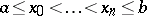 , and a set of
  (not necessarily different) values
  . Suppose that it is known that a function
  , belonging to some fixed class of functions
  that are defined at least on
  (e.g.,
  , where
  is the set of algebraic polynomials of degree
  , or
, or  ), satisfies the conditions
 | (i1) |
The points  at which the values
  are given are called the interpolation nodes, or interpolation knots, of
  . The following two problems arose naturally, mainly through the demands of numerical analysis. They were the starting point for the development of the theory of interpolation. It is asked, imposing (i1) on
  , how to obtain, with prescribed accuracy, information on the behaviour of
  : 1) on the intervals
  ,
,  , i.e. between (in Latin: inter) the nodes
  ,
,  ; and 2) outside (in Latin: extra) the interval
  containing all nodes
  . The Latin words "inter" and "extra" led, respectively, to the terminology of calling 1) an interpolation problem and 2) an extrapolation problem for the function
  ; these both were later merged into the one interpolation problem (i1).
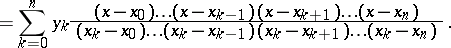
Problem (i1), regarded as the problem of exactly recovering functions, has a unique solution in, e.g., the class  . Its solution in
  is the Lagrange interpolation polynomial
 |
 |
However, if  belongs to a class that is in a certain sense "more extensive" than
  , problem (i1), in general, does not have, a unique solution. Nevertheless, the polynomial
  allows one to assess, to a certain extent, the behaviour of
  on
on  if it is considered that
 | (1) |
In relation to this it is necessary to estimate the error
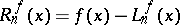 |
for  . The error depends mainly on the class
  to which
  belongs, in other words,
  depends on a priori known properties of
  . E.g., if
  , then the remainder term for (i1) has the form
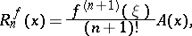 |
where  and
and
 |
Here  ,
,  denote, respectively, the minimum and maximum of the numbers
  ,
,  and
and  . The given formula for the remainder is due to A.L. Cauchy, cf. [3]. The quantity
  depends mainly on the form of the distribution and the number of interpolation nodes
  on
on  . It is in this connection natural to assume that the more interpolation nodes
  are taken and the more "uniformly" they are distributed on
  , then the more "accurate" relation (1) will be. This circumstance leads, in turn, to a more important interpolation problem, closely connected with (i1).
Suppose that  belongs to a class
  of functions that are defined on
  , and such that
  for all
  . It is assumed that the set of interpolation nodes
  ,
,  if
if  , is countable; suppose also that a sequence of values
  is given. The question is: How to recover
  from the given data:
 | (i2) |
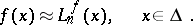
The problem posed in this way is in the general case far from solvable, and has to be made more precise. This will be done below, but now only a sketch of a very natural and important approach to solving (i2) will be given. Usually one first solves the "truncated" problem (i1):
 |
in  . Let
. Let  be the interpolation polynomial that is the solution to this truncated problem and let it be written as a Lagrange interpolation polynomial. Then one considers the possibility of accomplishing, in some sense or another, a limit
  as
as  (this is equivalent, in particular, to the study of the question of the remainder
  tending to zero as
  in the sense considered). The given sketch of the scheme for solving (i2) is fundamental for the theory of convergence (and divergence) of interpolation processes (cf. Interpolation process). It is one of the basic methods for solving interpolation problems and has applications not only in various branches of pure mathematics (e.g., number theory, cf. [3]), but also in numerical methods (cf. Interpolation in numerical mathematics, as well as [1]).
In the latter, along with interpolation problems of the kind considered above and defined by the simplest functionals  , one also started to study other problems, in which, e.g., the values of derivatives
  ,
,  , or more complicated functionals, are prescribed. In solving them one uses interpolation processes in which, instead of
  , other underlying interpolating sets of functions are considered, e.g. the class
  of trigonometric polynomials of degree
  , classes of rational functions
  (of the form
  , where
  and
and  ,
,  ), classes of entire functions of a special kind, etc. See also Interpolation formula.
In its general form, the problem of interpolation reads as follows. Let  ,
,  be two non-empty sets; suppose that a family of mappings
  ,
,  ,
,  , is given. Let
  be a given set of elements (not necessarily different) in
  . Then there naturally arises the problem of determining the set of
  satisfying
 | (i3) |
Generally speaking, not for every a priori given set of elements  does (i3) have a solution
  . Therefore, the formulated problem needs to be made more precise. This is done as follows.
1) Characterize the set  of sets
  for which the system of equations (i3) (which may be infinite) has at least one solution
  . In other words, it is required to give a constructive description of the set
  of all admissible sets
  , for a given fixed family of mappings
  , such that (i3) has a solution in
  .
.
2) Let  be a fixed admissible set of elements of
  (i.e. belonging to the set
  in 1) for (i3). It is required to find the set of all solutions
  of (i3).
When solving 1) or 2), answers to the following questions of a more particular nature are important.
3) What is the subset  on which (i3) has a unique solution
  for each admissible set
  for
for  with
with  ?
?
4) Let  be a subset of
  , usually only given by some restrictive property. It is required to give a constructive characterization of the set of solutions
  of (i3) under the condition that the right-hand side of (i3) "runs over"
  .
.
The specification of sets  ,
,  , families of mappings
  (
( for all
  ) together with the questions 1) and 2) (and usually with the related question 3), or sometimes 4)) determine the interpolation problem (i3). A class of problems of this kind is called a class of direct interpolation problems.
Each of the above problems 1)–4) is of scientific interest in itself. Problem 1) has a "multi-faceted character" : it is studied in number theory, functional analysis, function theory, etc. Suppose, e.g., that  is a real number,
  , and let
  be its fractional part. A family of mappings
  ,
,  , is given as follows:
  ,
,  ,
,  ,
,  and the following concrete version of the interpolation problem (i3) is considered:
 | (2) |
For certain subsets  one has investigated 1) for problem (2) to a certain extent. Problem (2) as a whole is difficult: Up till now (1978), e.g., no solution is known to the problem of the distribution of the fractional parts
  of powers of the number
  . This is a very particular subproblem of 1) for (2). A relation between 1) and the basis problem for systems of elements in various function spaces has been observed in, e.g., [9].
Problem 2) is the oldest of the theory of interpolation; it is the starting point of the theory of interpolation, and the names of I. Newton, J.L. Lagrange, N.H. Abel, Ch. Hermite, etc. are connected with it. Problems 1), 3) and 4) were not considered until the 20th century, while the solution to 2) was, as a rule, formal.
Problem 3) is closely related to 2), but is of interest only because in many problems it is equivalent to the completeness problem, and sometimes to the basis problem for various systems of elements  in corresponding function spaces. (Completeness is usually established by Banach's criterion, in which the equivalence of completeness problems with a certain uniqueness problem is shown.)
An important topic of research related to 4) is that of studying classes of functions taking integer values on a given set of points (e.g.,  or
or  ,
,  must be integers). This area was especially rapidly developed after the following result of G. Pólya: If an entire function
  of exponential type
  is such that its values
  ,
,  are integers, then
  is a polynomial. The constant
  in this theorem is best possible, since
  is an entire function of exponential type
  , which is different from a polynomial, and which takes integer values at
  (cf., e.g., [5], [10]).
If the set  in (i3) is a topological space and if a reduced problem (i3) (in some sense or another) has a solution
  , then one of the methods for solving it is an interpolation process in which the convergence of
  to the solution of (i3) is studied. Particular forms of processes of this kind can be found above. However, in many cases problems of type (i3) can be solved effectively by functional-analytic methods (cf., e.g., [10]).
Next to direct interpolation problems, inverse interpolation problems have some interest. The main contents of studies in this direction consist of the following.
Suppose that non-empty sets  ,
,  and a certain class
  of families of mappings
  acting from
  into
into  are given. Let
  be a certain family of sets of elements of
  . The problem is to find necessary and sufficient conditions on a subclass
  such that there is a family
  with the property that the set
  coincides with
  (or
(or  , or
, or  ) if
) if  runs over the entire set
  . The sets
  and
and  are strongly related to one another. Therefore it is usual in studies related to the branch of inverse interpolation problems to consider the pair
  as one entity. As an example of an inverse problem of the kind described above one may take one of the formulations of the circle of problems related to the well-known Nevanlinna–Pick interpolation problem: Let
  be a sequence of points in the open unit disc
  of the complex plane
  . Each function
  of class
  (
( is the class of bounded analytic functions in
  ) is associated with its sequence of values at
  :
:
 |
Thus, a certain kind of mappings  from
from  into
into  is given. Let
  be the space
  (of bounded sequences of complex numbers
  with norm
  ). In this case, the inverse problem has the following concrete form: Characterize the set of all sequences
  in
in  (i.e. of the class
  of mappings of the particular form
  ) with the property that the operator
  maps all of
  onto
onto  . Sequences
  with this property are called interpolating sequences. Thus, the set of all interpolating sequences
  determines the class
  in the given situation. The solution to this problem is Carleson's theorem: A sequence
  in
in  is interpolating if and only if a
  exists such that
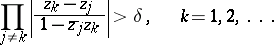 |
(the so-called separation condition). Inverse interpolation problems of the kind solved by L. Carleson have also been considered for other function classes and corresponding spaces of sequences of numbers (cf., e.g., [9], [12], [13], [14]).
See also Abel–Goncharov problem.
References
| [1] | I.S. Berezin, N.P. Zhidkov, "Computing methods" , Pergamon (1973) (Translated from Russian) |
| [2] | A.O. [A.O. Gel'fond] Gelfond, "Differenzenrechnung" , Deutsch. Verlag Wissenschaft. (1958) (Translated from Russian) |
| [3] | V.L. Goncharov, "The theory of interpolation and approximation of functions" , Moscow (1954) (In Russian) |
| [4] | J.L. Walsh, "Interpolation and approximation by rational functions in the complex domain" , Amer. Math. Soc. (1969) |
| [5] | L. Bieberbach, "Analytische Fortsetzung" , Springer (1955) pp. Sect. 3 |
| [6] | N.E. Nörlund, "Volesungen über Differenzenrechnung" , Springer (1924) |
| [7] | N.E. Nörlund, "Leçons sur les séries d'interpolation" , Gauthier-Villars (1926) |
| [8] | J.M. Whittaker, "Interpolatory function theory" , Cambridge Univ. Press (1935) |
| [9] | P.L. Duren, "Theory of  spaces" , Acad. Press (1970) spaces" , Acad. Press (1970) |
| [10] | Yu.A. Kaz'min, "Interpolation methods for analytic functions and their applications" , Moscow (1972) (In Russian) (Thesis) |
| [11a] | Yu.F. Korobeinik, "On a dual problem 1. General results. Application to Fréchet spaces" Math. USSR Sb. , 26 (1975) pp. 181–212 Mat. Sb. , 97 : 2 (1975) pp. 193–229 |
| [11b] | Yu.F. Korobeinik, "On a dual problem 2. Applications to  -spaces and other questions" Math. USSR Sb. , 27 (1976) pp. 1–22 Mat. Sb. , 98 : 1 (1975) pp. 3–26 -spaces and other questions" Math. USSR Sb. , 27 (1976) pp. 1–22 Mat. Sb. , 98 : 1 (1975) pp. 3–26 |
| [12] | V. Kabaila, "Interpolation sequences for the  classes in case classes in case  " Litovsk. Mat. Sb. , 3 : 1 (1963) pp. 141–147 (In Russian) " Litovsk. Mat. Sb. , 3 : 1 (1963) pp. 141–147 (In Russian) |
| [13] | A.M. [A.M. Sedletskii] Sedleckii, "Interpolation in  spaces over a half-plane" Soviet Math. Dokl. , 14 (1973) pp. 276–278 Dokl. Akad. Nauk. SSSR , 208 : 6 (1973) pp. 1293–1295 spaces over a half-plane" Soviet Math. Dokl. , 14 (1973) pp. 276–278 Dokl. Akad. Nauk. SSSR , 208 : 6 (1973) pp. 1293–1295 |
| [14] | S.V. Shvedenko, "The interpolation of  sequences by sequences by  functions" Math. Notes , 21 (1977) pp. 281–284 Mat. Zametki , 21 : 4 (1977) pp. 503–508 functions" Math. Notes , 21 (1977) pp. 281–284 Mat. Zametki , 21 : 4 (1977) pp. 503–508 |
Comments
The topic of interpolation is a vast one, and is the subject of numerous papers and several treatises. It also includes e.g. interpolation by (all kinds of) spline functions [a4] and so-called Birkhoff interpolation (cf. Interpolation process) [a3]. Interpolation in several variables has also been studied in detail (cf. [a2]).
More on interpolating sequences can be found in, e.g., [a5]. See also Pick theorem; Nevanlinna–Pick problem.
References
| [a1] | L. Carleson, "An interpolation problem for bounded analytic functions" Amer. J. Math. , 80 (1958) pp. 921–930 |
| [a2] | P.R. Graves-Morris (ed.) E.B. Saff (ed.) R.S. Varga (ed.) , Rational Approximation and Interpolation (Tampa, 1983) , Lect. notes in math. , 1105 , Springer (1984) |
| [a3] | G.G. Lorentz, K. Jetter, S.D. Riemenschneider, "Birkhoff interpolation" , Wiley (1983) |
| [a4] | L.L. Schumaker, "Spline functions, basic theory" , Wiley (1981) |
| [a5] | J.B. Garnett, "Bounded analytic functions" , Acad. Press (1984) |
Interpolation. Encyclopedia of Mathematics. URL: http://encyclopediaofmath.org/index.php?title=Interpolation&oldid=19144