Singular integral equation
An equation containing the unknown function under the integral sign of an improper integral in the sense of Cauchy (cf. Cauchy integral). Depending on the dimension of the manifold over which the integrals are taken, one distinguishes one-dimensional and multi-dimensional singular integral equations. In comparison with the theory of Fredholm equations (cf. Fredholm equation), the theory of singular integral equations is more complex. For example, the theories of one-dimensional and multi-dimensional singular integral equations, both in the formulation of definitive results and in the methods used to establish them, differ significantly from one another. In the one-dimensional case, the theory is more fully developed, and its results are formulated more simply than the corresponding results in the multi-dimensional case. In what follows, main attention will be given to the one-dimensional case.
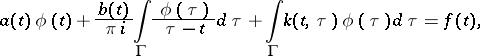
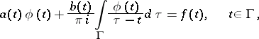
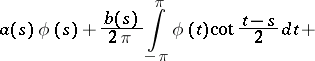
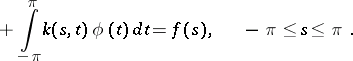
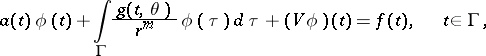
An important class of one-dimensional singular integral equations are those with a Cauchy kernel:
 | (1) |
 |
where  ,
,  ,
,  ,
,  are known functions,
  is a Fredholm kernel (see Integral operator),
  is the desired function,
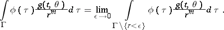
  is a planar curve, and the improper integral is to be understood as a Cauchy principal value, i.e.
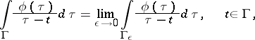 |
where  ,
,  being the arc
  on
on  such that
  and
and  are both of length
  .
.
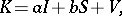
The operator  defined by the left-hand side of (1) is called a singular operator (or sometimes a general singular operator):
 | (2) |
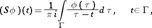
where  is the identity operator,
  is a singular integral operator (sometimes called a singular integral operator with Cauchy kernel), i.e.
 |
and  is the integral operator with kernel
  .
.
The operator  is called the characteristic part of the singular operator
  , or the characteristic singular operator, and the equation
 | (3) |
is called a characteristic singular integral equation, the functions  and
and  being the coefficients of the corresponding operator or equation.
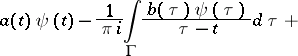
The equation
 |
 |
is called the adjoint of equation (1), and the operator 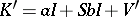 (
( being the integral operator with kernel
  ) is called the adjoint of
  . In particular,
 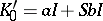 is the adjoint of
  .
.
The operators  ,
,  ,
,  ,
,  , or their corresponding equations, are said to be of normal type if the functions
 |
do not vanish anywhere on  . In this case one also says that the coefficients of the operator or equation satisfy the normality condition.
Let  ,
,  , be the class of functions
  defined on
  and satisfying the condition
 |
for all  . If
. If  belongs to
  for some admissible value
  and knowledge of the numerical value of
  is not required, then one writes
  , or even
  if it is clear from the context which contour
  is meant.
The set  is called a Hölder class of functions, and if
  one says that
  satisfies a Hölder condition or that
  is an
is an  -function.
Let  be a complex-valued continuous function that does not vanish on an oriented closed simple smooth contour
  , and let
 | (4) |
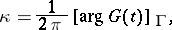
where  denotes the increment of the function between brackets after a single circuit of
  in the positive direction. The integer
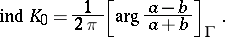
  is called the index of the function
  ,
,  .
.
Solution of the characteristic singular integral equation and its adjoint.
Let  be a simple, closed, oriented, smooth contour on which the positive direction is chosen in such a way that it bounds a finite domain on the left, let the coordinate origin lie in this domain, let
  , and let
  and
and  satisfy the normality condition. Further, let
  be defined by (4), with
 | (5) |
Then the following assertions hold.
1) If  , then the equation (3) is solvable in
  for any right-hand side
  , and all its
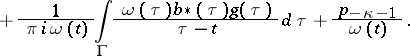
  -solutions are given by the formula (see [1], [2])
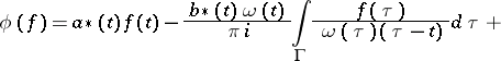 | (6) |
 |
where
 |
 |
and  is an arbitrary polynomial of degree
  (
( ). If
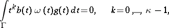
). If  , then equation (3) is solvable in
  if and only if
  satisfies the condition
 |
When these conditions hold, (3) has a unique  -solution, given by the formula (6) with
  .
.
2) The singular integral equation adjoint to (3),
 | (7) |
is solvable in  for any
  if
if  , and all its
  -solutions are given by the formula
 | (8) |
 |
But if  , equation (7) is solvable if and only if
  satisfies the
  conditions:
 |
and if these conditions hold, the solution is given by (8) with  .
.
Noether's theorems. Let  and
and  be the numbers of linearly independent solutions of the homogeneous equations
  and
and  , respectively. Then the difference
  is called the index of the operator
  or of the equation
  :
:
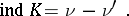 |
Theorem 1.
The homogeneous singular integral equations  and
and  have a finite number of linearly independent solutions.
Theorem 2.
Necessary and sufficient conditions for the solvability of the non-homogeneous equation (3) are:
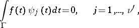 |
where  is a complete set of linearly independent solutions of the adjoint homogeneous equation
  .
.
Theorem 3.
The index of  (cf. Index of an operator) is equal to the index of the function
  defined by equation (5), i.e.
 | (9) |
These theorems remain valid in the case of the general singular integral equation (1), that is, in these theorems  ,
,  can be replaced by
  ,
,  , respectively. It is only necessary to bear in mind that, in the case of general singular integral equations,
  and
and  are both non-zero in general, in contrast to the case of characteristic singular integral equations, when one of them must be zero.
Theorems 1–3 are called after F. Noether, who first proved them [9] in the case of a one-dimensional singular integral equation with Hilbert kernel:
 | (10) |
 |
These theorems are analogous to the Fredholm theorems (see Fredholm equation) and differ from them only in that the numbers of linearly independent solutions of the homogeneous equation and its adjoint are in general distinct, that is, whereas the index of a Fredholm equation is always equal to zero, a singular integral equation can have non-zero index.
Like the Noether theorems, the formulas (6) and (8) remain valid in the case when  consists of a finite number of smooth mutually-disjoint closed contours. In this case the symbol
  in (4) denotes the sum of the increments of the function between brackets after a circuit of each of the contours
  .
.
The case when  is a finite union of smooth mutually-disjoint open contours requires special consideration. If
  is an
is an  -function inside any closed part of every
  not containing the end points, and if close to either end
  it can be written in the form
 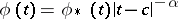 ,
,  , where
  is an
is an  -function in a neighbourhood of
  containing
  , then one says that
  belongs to the class
  . If
. If  ,
,  and in
  one looks for solutions of the equations (3), (7), then one can define
  and
and  in such a way that (6) and (8) remain valid. Furthermore, if one defines in a corresponding way subclasses of
  in which one looks for solutions of a given singular integral equation and its adjoint, then the Noether theorems also remain valid (see [1]).
The above results can be extended in various ways. It can be shown (see [1]) that under certain conditions they also remain valid in the case of a piecewise-smooth contour  (that is, when
  is the union of a finite number of smooth open arcs, which are mutually-disjoint except for their end points). Singular integral equations can also be studied in the Lebesgue function spaces
  and
and  , where
  and
and  is a certain weight (see [4]–[7]). [4]–[6] contain results which directly extend those stated above.
Let  be a simple rectifiable contour with equation
  ,
,  , where
  is the arc-length on
  starting from some fixed point and
  is the length of
  . One says that a function
  defined on
  is almost-everywhere finite, measurable, integrable, etc., if the function
  has the corresponding property on the interval
  . The Lebesgue integral of
  on
on  is defined by
 |
Let  denote the set of measurable functions on
  such that
  is integrable on
  . The function class
  ,
,  , becomes a Banach space if one introduces the norm by
 |
If in equations (3), (7) the equalities hold almost-everywhere, with continuous coefficients  and
and  satisfying the normality condition and
  ,
,  , then 1) and 2) remain valid upon replacing
  by
by  ,
,  . Furthermore, if the solutions of
  , where
  has the form (2), are sought in
  ,
,  , and the solutions of its homogeneous adjoint
  are sought in
  , where
  , then the Noether theorems also remain valid and
  may be any completely-continuous operator on
  .
.
When  is a finite union of open contours, or if
  is closed but the coefficients of the singular integral equation are not continuous, then solutions of the equations can often be found in weighted function spaces
  ,
,  (
( ). Under specific conditions on the weight function
  , results analogous to the above are valid.
The regularization problem.
One of the basic problems in the theory of singular integral equations is the regularization problem, that is, the problem of reducing a singular integral equation to a Fredholm equation.
Let  and
and  be Banach spaces, which may coincide, and let
  be a bounded linear operator. A bounded operator
  is called a left regularizer of
  if
if  , where
  ,
,  are the identity and a completely-continuous operator on
  , respectively. If the equations
  and
and  are equivalent for each
  , then
  is called a left equivalent regularizer of
  . A bounded operator
  is called a right regularizer of
  if
if  , where
  ,
,  are the identity and a completely-continuous operator on
  , respectively. If the equations
  and
and  are simultaneously solvable or unsolvable as
  ranges over
  , and in the case of solvability the relation
  holds between their solutions, then
  is called a right equivalent regularizer of
  . If
. If  is simultaneously a left and right regularizer of
  , then it is called a two-sided regularizer, or simply a regularizer of
  . One says that
  admits left, right, two-sided, equivalent, regularization if it has a left, right, two-sided, or equivalent regularizer, respectively.
Let  be the operator defined by (2), where
  is a closed simple smooth contour,
  and
and  are
are  -functions (or continuous functions) satisfying the normality condition and
  is a completely-continuous operator on
  ,
,  . Then
  has an uncountable set of regularizers on
  , e.g. one of which is the operator
 |
For  to admit left equivalent regularization, it is necessary and sufficient that its index
  is non-negative [7]. One can take
  to be an equivalent left regularizer. If
  , then
  admits right equivalent regularization, which can be realized using
  (see [1]).
Systems of singular integral equations.
If in (1)  ,
,  and
and  are square matrices of order
  , regarded as matrices of linear transformations of an unknown vector
  , and
, and  is a known vector, then (1) is called a system of singular integral equations. It is said to be of normal type if the matrices
  and
and  are non-singular on
  , that is,
  and
and  for all
  .
.
The Noether theorems remain valid for a system of singular integral equations in the class  (see [1], [3]), and can be extended to the case of Lebesgue function spaces (see [4], [5]). In contrast to the case of a single equation, a characteristic system of singular integral equations cannot, in general, be solved by quadratures, although there is a formula similar to (9) for the index (see [1]):
 |
For a system of singular integral equations, regularization problems (see [3]) are similar to those for a single equation.
There have been several investigations of both one singular integral equation and a system of such equations when the normality condition is violated (see [11] and the bibliography contained therein).
Multi-dimensional singular integral equations.
These are equations of the form
 | (11) |
where  is a domain in the Euclidean space
  ,
,  .
.  may be bounded or unbounded, and can, in particular cases, coincide with
  ;
;  and
and  are points of
  ,
,  ,
,  ,
,  is the volume element in
  , and
, and  is a completely-continuous operator on the Banach function space in which the solution is sought. Further,
  and
and  are given functions and the improper singular integral is understood in the principle value sense, that is,
 | (12) |
Here  is called the pole,
  the characteristic and
  the density of the singular integral (12). As a rule, the limit in (12) does not exist when the following condition is violated:
 | (13) |
where  is the unit sphere with centre at the origin. Thus it is assumed that (13) always holds.
In the theory of multi-dimensional singular integral equations, an important role is played by the notion of a symbol (cf. Symbol of an operator). It is defined in terms of the functions  and
and  , and from a given symbol the original singular operator can be recovered up to a completely-continuous term. Composition of singular operators corresponds to multiplication of their symbols. It has been shown [7] that under certain restrictions (11) admits a regularization in the space
  ,
,  , if and only if the absolute value of its symbol has a positive lower bound, and in this case the Fredholm theorems hold.
Historical survey.
The study of one-dimensional singular integral equations originated in the works of D. Hilbert and H. Poincaré at almost the same time as the formulation of the theory of Fredholm equations (cf. Fredholm equation). A special case, a singular integral equation with Cauchy kernel, was considered much earlier in the doctoral thesis of Yu.V. Sokhotskii, published in St. Petersburg in 1873; however, this research remained unnoticed.
Basic results on the formulation of a general theory of the equations (1) and (10) were obtained at the beginning of the 1920s by Noether [9] and T. Carleman [10]. Noether first introduced the concept of an index and proved the theorems 1–3 above by applying the method of left regularization. This method was first described (in various special cases) by Poincaré and Hilbert, but its general form is due to Noether. A crucial point in the realization of the above method involves the application of a permutation (composition) formula for repeated singular integrals in the Cauchy principal value sense (the Poincaré–Bertrand formula). For certain special classes of equations (3), Carleman had the basic idea behind a method for reducing this equation to the following boundary value problem in the theory of analytic functions (the linear conjugacy problem, see [1] and Riemann–Hilbert problem (analytic functions)):
 |
and found a way of constructing an explicit solution. Carleman and I.N. Vekua found a method of regularizing equation (1) involving a solution of the characteristic equation (3).
The great significance, both theoretical and practical, of singular integral equations became especially apparent towards the end of the 1930s in connection with the solution of certain very important problems in the mechanics of a solid medium (the theory of elasticity, hydro- and aeromechanics, and others) and theoretical physics. The theory of one-dimensional singular integral equations was significantly advanced in the 1940s and reached a final form (in a definite sense) in the works of Soviet mathematicians. A presentation of this theory in Hölder classes of functions is to be found in a monograph of one of its creators, N.I. Muskhelishvili (see [1]). This monograph also stimulated scientific investigations in certain other directions, for example in the theory of singular integral equations not satisfying the Hausdorff normality condition, singular integral equations with non-diagonal singularities (with displacements), Wiener–Hopf equations, multi-dimensional singular integral equations, etc.
The earliest studies of multi-dimensional singular integral equations were carried out in 1928 by F. Tricomi, who established a permutation formula for two-dimensional singular integrals and applied it to the solution of a class of singular integral equations. In this direction, the fundamental work was done in 1934 by G. Giraud, who proved the validity of the Fredholm theorems for certain classes of multi-dimensional singular integral equations on Lyapunov manifolds.
References
| [1] | N.I. Muskhelishvili, "Singular integral equations" , Wolters-Noordhoff (1972) (Translated from Russian) |
| [2] | F.D. Gakhov, "Boundary value problems" , Pergamon (1966) (Translated from Russian) |
| [3] | N.P. Vekua, "Systems of singular integral equations and some boundary value problems" , Moscow (1970) (In Russian) |
| [4] | B.V. Khvedelidze, "Linear discontinuous boundary problems in the theory of functions, singular integral equations and some applications" Trudy Tbilis. Mat. Inst. Akad. Nauk. GruzSSR , 23 (1956) pp. 3–158 (In Russian) |
| [5] | I.I. Danilyuk, "Nonregular boundary value problems on the plane" , Moscow (1975) (In Russian) |
| [6] | I. [I.Ts. Gokhberg] Gohberg, N. Krupnik, "Einführung in die Theorie der eindimensionalen singulären Integraloperatoren" , Birkhäuser (1979) (Translated from Russian) |
| [7] | S.G. Mikhlin, "Multidimensional singular integrals and integral equations" , Pergamon (1965) (Translated from Russian) |
| [8] | A.V. Bitsadze, "Boundary value problems for second-order elliptic equations" , North-Holland (1968) (Translated from Russian) |
| [9] | F. Noether, "Ueber eine Klasse singulärer Integralgleichungen" Math. Ann. , 82 (1921) pp. 42–63 |
| [10] | T. Carleman, "Sur le résolution des certaines équations intégrales" Arkiv. Mat. Astron. Fys. , 16 : 26 (1922) pp. 1–19 |
| [11] | S. Prössdorf, "Einige Klassen singulärer Gleichungen" , Birkhäuser (1974) |
Comments
For certain systems of singular integral equations explicit solution formulas can be obtained by using the state-space approach from systems theory (cf. [a1] and Integral equation of convolution type).
References
| [a1] | H. Bart, I. Gohberg, M.A. Kaashoek, "Minimal factorization of matrix and operation functions" , Birkhäuser (1979) |
| [a2] | K. Clancey, I. Gohberg, "Factorization of matrix functions and singular integral operators" , Birkhäuser (1981) |
Singular integral equation. Encyclopedia of Mathematics. URL: http://encyclopediaofmath.org/index.php?title=Singular_integral_equation&oldid=11918