Difference between revisions of "Variational calculus, numerical methods of"
(Importing text file) |
Ulf Rehmann (talk | contribs) m (tex encoded by computer) |
||
| Line 1: | Line 1: | ||
| + | <!-- | ||
| + | v0962101.png | ||
| + | $#A+1 = 135 n = 0 | ||
| + | $#C+1 = 135 : ~/encyclopedia/old_files/data/V096/V.0906210 Variational calculus, numerical methods of | ||
| + | Automatically converted into TeX, above some diagnostics. | ||
| + | Please remove this comment and the {{TEX|auto}} line below, | ||
| + | if TeX found to be correct. | ||
| + | --> | ||
| + | |||
| + | {{TEX|auto}} | ||
| + | {{TEX|done}} | ||
| + | |||
The branch of numerical mathematics in which one deals with the determination of extremal values of functionals. | The branch of numerical mathematics in which one deals with the determination of extremal values of functionals. | ||
| Line 10: | Line 22: | ||
With the advent of the Pontryagin maximum principle (1956), variational problems can very often be reduced to boundary value problems. | With the advent of the Pontryagin maximum principle (1956), variational problems can very often be reduced to boundary value problems. | ||
| − | Consider the following problem in optimal control: Find a trajectory | + | Consider the following problem in optimal control: Find a trajectory $ x( t) $ |
| + | and a control $ u( t) $ | ||
| + | for which the functional | ||
| − | + | $$ \tag{1 } | |
| + | J = \int\limits _ {t _ {0} } ^ { T } f ^ { 0 } ( t, x, u) dt | ||
| + | $$ | ||
assumes its minimal value, given the differential constraints | assumes its minimal value, given the differential constraints | ||
| − | + | $$ \tag{2 } | |
| + | \dot{x} = f ( t, x, u), | ||
| + | $$ | ||
the boundary conditions | the boundary conditions | ||
| − | + | $$ \tag{3 } | |
| + | x ( t _ {0} ) = x _ {0} , | ||
| + | $$ | ||
| − | + | $$ \tag{4 } | |
| + | x ( T) = x _ {T} , | ||
| + | $$ | ||
and control restrictions | and control restrictions | ||
| − | + | $$ \tag{5 } | |
| + | u \in U, | ||
| + | $$ | ||
| − | where | + | where $ x = ( x ^ {1} \dots x ^ {n} ) $, |
| + | $ u = ( u ^ {1} \dots u ^ {m} ) $ | ||
| + | are the vectors of the coordinates of the phase and the controls, $ f = ( f ^ { 1 } \dots f ^ { n } ) $, | ||
| + | $ U $ | ||
| + | is a closed set in an $ m $- | ||
| + | dimensional space, and $ t $( | ||
| + | the time) is an independent variable. | ||
| − | According to Pontryagin's maximum principle, the optimal control | + | According to Pontryagin's maximum principle, the optimal control $ u( t) $ |
| + | must, for any $ t $, | ||
| + | produce the absolute maximum of the [[Hamilton function|Hamilton function]] | ||
| − | + | $$ \tag{6 } | |
| + | H ( {\widetilde{u} } ) = \max _ {u \in U } H ( u) = | ||
| + | $$ | ||
| − | + | $$ | |
| + | = \ | ||
| + | \max _ {u \in U } \left [ \sum _ {i = 1 } ^ { n } \psi _ {i} f ^ { i } ( t, x, u) - f ^ { 0 } ( t, x, u) \right ] , | ||
| + | $$ | ||
| − | where | + | where $ \psi = ( \psi _ {1} \dots \psi _ {n} ) $ |
| + | is defined by the system of equations | ||
| − | + | $$ \tag{7 } | |
| + | \dot \psi _ {i} = - | ||
| + | \frac{\partial H }{\partial x ^ {i} } | ||
| + | ,\ \ | ||
| + | i = 1 \dots n. | ||
| + | $$ | ||
| − | The control | + | The control $ u( t, x, \psi ) $ |
| + | is found from condition (6) and is substituted in (2) and (7). As a result one obtains a closed boundary value problem for a system of $ 2n $ | ||
| + | differential equations (2) and (7) with $ 2n $ | ||
| + | boundary conditions (3) and (4). | ||
The scheme of numerical solution which is most frequently employed for this boundary value problem involves the use of Newton's method of fractional steps [[#References|[3]]]. One introduces the discrepancy vector | The scheme of numerical solution which is most frequently employed for this boundary value problem involves the use of Newton's method of fractional steps [[#References|[3]]]. One introduces the discrepancy vector | ||
| − | + | $$ \tag{8 } | |
| + | \phi _ {i} = x ^ {i} ( T) - x _ {T} ^ {i} ,\ \ | ||
| + | i = 1 \dots n, | ||
| + | $$ | ||
| − | where the value of | + | where the value of $ x ^ {i} ( T) $ |
| + | is obtained by solving the Cauchy problem for the system (2), (7) with initial conditions (3) and $ \psi _ {j} ( t _ {0} ) = \psi _ {j0} $, | ||
| + | $ j = 1 \dots n $. | ||
| + | The discrepancies (8) are considered as functions of the unknowns $ \psi _ {10} \dots \psi _ {n0} $, | ||
| + | defined by the system of equations | ||
| − | + | $$ \tag{9 } | |
| + | \phi _ {i} ( \psi _ {10} \dots \psi _ {n0} ) = 0,\ \ | ||
| + | i = 1 \dots n. | ||
| + | $$ | ||
The system (9) is solved by Newton's method (cf. [[Newton method|Newton method]]); the partial derivatives involved, | The system (9) is solved by Newton's method (cf. [[Newton method|Newton method]]); the partial derivatives involved, | ||
| − | + | $$ | |
| + | |||
| + | \frac{\partial \phi _ {i} }{\partial \psi _ {j0} } | ||
| + | ,\ \ | ||
| + | i, j = 1 \dots n, | ||
| + | $$ | ||
are numerically determined by the formula: | are numerically determined by the formula: | ||
| − | + | $$ | |
| − | + | \frac{\partial \phi _ {i} }{\partial \psi _ {j0} } | |
| + | \approx | ||
| + | $$ | ||
| − | + | $$ | |
| + | \approx \ | ||
| − | + | \frac{\phi _ {i} ( \psi _ {10} \dots \psi _ {j0} + \Delta \psi _ {j0} \dots \psi _ {n0} ) - \phi _ {i} ( \psi _ {10} \dots \psi _ {n0} ) }{\Delta \psi _ {j0} } | |
| + | , | ||
| + | $$ | ||
| − | where | + | where the values of $ \phi _ {i} ( \psi _ {10} \dots \psi _ {j0} + \Delta \psi _ {j0} \dots \psi _ {n0} ) $ |
| + | are obtained by solving Cauchy's problem for the system (2), (7), with initial conditions (3) and conditions | ||
| − | + | $$ | |
| + | \psi _ {l} ( t _ {0} ) = \psi _ {l _ {0} } ,\ \ | ||
| + | \psi _ {j} ( t _ {0} ) = \psi _ {j0} + \Delta \psi _ {j0} ,\ \ | ||
| + | l \neq j, | ||
| + | $$ | ||
| − | The difficulties in Newton's method consist, in the first place, in the selection of a successful initial approximation for | + | where $ \Delta \psi _ {j0} $ |
| + | is a small increment of $ \psi _ {j0} $. | ||
| + | |||
| + | The partial derivatives may be determined by a more accurate, but more laborious, method [[#References|[4]]], involving the integration of a system of $ 2n $ | ||
| + | equations in variations for the system (2), (7). | ||
| + | |||
| + | The difficulties in Newton's method consist, in the first place, in the selection of a successful initial approximation for $ \psi _ {j0} $ | ||
| + | and, secondly, in the unstability of the Cauchy problem, which is very strongly manifested on large intervals $ [ t _ {0} , t _ {1} ] $. | ||
| + | There is no generally valid procedure to overcome the first difficulty. A number of methods (cf. [[Cauchy problem, numerical methods for ordinary differential equations|Cauchy problem, numerical methods for ordinary differential equations]]) are available to deal with the unstability of the Cauchy problem. | ||
If the boundary conditions and the functional are given in a more general form than in (3), (4) and (1) (e.g. in the [[Bolza problem|Bolza problem]] with mobile ends, in a [[Variational problem|variational problem]] with free (mobile) ends), the [[Transversality condition|transversality condition]] is added to supplement the optimality conditions (6) and (7). After elimination of the arbitrary constants which appear in these conditions, a closed boundary value problem and a corresponding system of equations of the type (9) are obtained. | If the boundary conditions and the functional are given in a more general form than in (3), (4) and (1) (e.g. in the [[Bolza problem|Bolza problem]] with mobile ends, in a [[Variational problem|variational problem]] with free (mobile) ends), the [[Transversality condition|transversality condition]] is added to supplement the optimality conditions (6) and (7). After elimination of the arbitrary constants which appear in these conditions, a closed boundary value problem and a corresponding system of equations of the type (9) are obtained. | ||
| Line 81: | Line 160: | ||
The first direct method was proposed by Euler for the solution of the simplest problem in variational calculus. It is known as Euler's method of polygonal lines (or as Euler's finite-difference method). In this method the functional | The first direct method was proposed by Euler for the solution of the simplest problem in variational calculus. It is known as Euler's method of polygonal lines (or as Euler's finite-difference method). In this method the functional | ||
| − | + | $$ \tag{10 } | |
| + | J ( x) = \ | ||
| + | \int\limits _ { t _ {0} } ^ { {t _ 1 } } | ||
| + | F ( t, x, \dot{x} ) dt | ||
| + | $$ | ||
| − | is considered on continuous polygonal lines | + | is considered on continuous polygonal lines $ x( t) $ |
| + | which satisfy given boundary conditions | ||
| − | + | $$ \tag{11 } | |
| + | x ( t _ {0} ) = x _ {0} ,\ \ | ||
| + | x ( t _ {1} ) = x _ {1} , | ||
| + | $$ | ||
| − | and which consist of | + | and which consist of $ N $ |
| + | rectilinear segments with end points at given abscissas. Thus, the functional becomes a function of the ordinates of the vertices of the polygonal line, while the initial problem is reduced to the task of minimizing a function of several variables (cf. [[Euler method|Euler method]]). | ||
Since the labour involved in such calculations is considerable, direct methods were neglected for a long time in traditional studies in variational calculus. They were taken up again early in the 20th century. New methods for the reduction to the problem of finding an extremum of a function of several variables were proposed. Of these, the most important one is the [[Ritz method|Ritz method]], according to which the solution of minimizing (10) subject to condition (11) is to be found in the class of functions of the form | Since the labour involved in such calculations is considerable, direct methods were neglected for a long time in traditional studies in variational calculus. They were taken up again early in the 20th century. New methods for the reduction to the problem of finding an extremum of a function of several variables were proposed. Of these, the most important one is the [[Ritz method|Ritz method]], according to which the solution of minimizing (10) subject to condition (11) is to be found in the class of functions of the form | ||
| − | + | $$ | |
| + | x = \phi _ {0} ( t) + \sum _ {i = 1 } ^ { N } a _ {i} \phi _ {i} ( t), | ||
| + | $$ | ||
| − | where | + | where $ {\phi _ {i} } ( t) $, |
| + | $ i = 0 \dots N $, | ||
| + | are elements of a complete infinite system of linearly independent functions which satisfy the boundary conditions | ||
| − | + | $$ | |
| + | \phi _ {0} ( t _ {0} ) = x _ {0} ,\ \ | ||
| + | \phi _ {0} ( t _ {1} ) = x _ {1} ,\ \ | ||
| + | \phi _ {i} ( t _ {0} ) = \phi _ {i} ( t _ {1} ) = 0, | ||
| + | $$ | ||
| − | + | $$ | |
| + | i = 1, 2 ,\dots. | ||
| + | $$ | ||
The problem is reduced to finding a minimum of the function | The problem is reduced to finding a minimum of the function | ||
| − | + | $$ | |
| + | J = J ( a _ {1} \dots a _ {N} ) | ||
| + | $$ | ||
| − | of | + | of $ N $ |
| + | variables. Ritz's method is sufficiently general. It is applied to the solution of variational problems in mathematical physics consisting of the minimization of a functional which depends on functions of several variables. A further generalization of the method to include this class of problems is the method, [[#References|[2]]], in which the coefficients are considered to be unknown functions of one of the independent variables (e.g. if the problem involves two independent variables $ t $ | ||
| + | and $ \tau $, | ||
| + | $ a _ {i} $ | ||
| + | may be given as $ {a _ {i} } ( \tau ) $). | ||
| + | The initial functional becomes dependent on $ N $ | ||
| + | functions $ {a _ {i} } ( \tau ) $, | ||
| + | which may be defined in terms of the necessary conditions, i.e., in the final count, by solving the boundary value problem for a system of $ N $ | ||
| + | Euler equations. | ||
Practical requirements enhanced the interest in non-classical problems of optimal control. The presence in technical problems of complicated restrictions on the phase coordinates and the control functions, the discontinuity of the right-hand sides of differential equations, the possible existence of singular and sliding optimal conditions, etc. — all this stimulated the development of new direct methods. The most popular methods are those involving the idea of descent in the space of controls and of successive analysis of variants (of the type of [[Dynamic programming|dynamic programming]]). | Practical requirements enhanced the interest in non-classical problems of optimal control. The presence in technical problems of complicated restrictions on the phase coordinates and the control functions, the discontinuity of the right-hand sides of differential equations, the possible existence of singular and sliding optimal conditions, etc. — all this stimulated the development of new direct methods. The most popular methods are those involving the idea of descent in the space of controls and of successive analysis of variants (of the type of [[Dynamic programming|dynamic programming]]). | ||
| − | Descent methods in the space of the controls are based on finding a sequence of controls | + | Descent methods in the space of the controls are based on finding a sequence of controls $ u _ {k} \in U $ |
| + | of the form | ||
| − | + | $$ \tag{12 } | |
| + | u _ {k + 1 } ( t) = \ | ||
| + | u _ {k} ( t) + \delta u _ {k} ( t), | ||
| + | $$ | ||
which corresponds to a monotone decreasing sequence of values of the functional. For instance, suppose it is required to find a minimum of the functional | which corresponds to a monotone decreasing sequence of values of the functional. For instance, suppose it is required to find a minimum of the functional | ||
| − | + | $$ \tag{13 } | |
| + | J = F ( x ( T)) | ||
| + | $$ | ||
| − | subject to the conditions (2), (3) and (5) ( | + | subject to the conditions (2), (3) and (5) ( $ U $ |
| + | is a convex and simply-connected set). The increment $ \delta u _ {k} ( t) $ | ||
| + | is found as follows. The variational equations for (2) and the conjugate system (7), subject to the conditions | ||
| − | + | $$ | |
| + | \psi _ {i} ( T) = \ | ||
| + | - | ||
| + | \frac{\partial F ( x ( T)) }{\partial x ^ {i} } | ||
| + | ,\ \ | ||
| + | i = 1 \dots n, | ||
| + | $$ | ||
| − | at the right-hand end, are used to represent the linear part of the increment of the functional (13) as a result of the variation | + | at the right-hand end, are used to represent the linear part of the increment of the functional (13) as a result of the variation $ \delta u $, |
| + | in the form | ||
| − | + | $$ | |
| + | \delta J = - \int\limits _ {t _ {0} } ^ { {T } } | ||
| + | |||
| + | \frac{\partial H }{\partial u } | ||
| + | |||
| + | \delta u dt. | ||
| + | $$ | ||
In order to decrease the value of the functional (13), the increment | In order to decrease the value of the functional (13), the increment | ||
| − | + | $$ | |
| + | \delta u _ {k} ( t) = \ | ||
| + | \kappa | ||
| + | \frac{\partial H }{\partial u } | ||
| + | ,\ \ | ||
| + | \kappa > 0, | ||
| + | $$ | ||
| − | where the value of | + | where the value of $ \partial H / \partial u $ |
| + | is calculated on the control $ {u _ {k} } ( t) $ | ||
| + | and on the corresponding trajectory $ {x _ {k} } ( t) $, | ||
| + | must be chosen for each iteration. The regularity of the linearization, and hence also the decrease in the value of the functional (13), is ensured by choosing a sufficiently small value of $ \kappa $. | ||
| + | The descent process (12) begins from some $ {u _ {0} } ( t) $ | ||
| + | and is terminated when, as a result of the last iteration, $ | \delta J | $ | ||
| + | becomes smaller than some given $ \epsilon $. | ||
| + | In the case of a free right-hand end described above, the resulting algorithm is most simple [[#References|[5]]], [[#References|[6]]], [[#References|[7]]]. Another method which does not involve linearization of the initial problem is very effective in solving problems with a free end [[#References|[8]]]. If the right-hand end is also subject to boundary conditions, all algorithms become much more complicated. To deal with boundary conditions, a gradient projection procedure is employed in [[#References|[5]]], while in [[#References|[6]]] failure to satisfy the boundary conditions is penalized by considering the functional | ||
| − | + | $$ \tag{14 } | |
| + | J = F( x( T)) + | ||
| + | \sum _ {i = 1 } ^ { n } | ||
| + | \lambda _ {i} ( x ^ {i} ( T) - x _ {T} ^ {i} ) ^ {2} ,\ \ | ||
| + | \lambda _ {i} > 0, | ||
| + | $$ | ||
rather than (13). The method in which the increment of the control is determined by solving an auxiliary linear programming problem, resembles the gradient methods [[#References|[9]]]. | rather than (13). The method in which the increment of the control is determined by solving an auxiliary linear programming problem, resembles the gradient methods [[#References|[9]]]. | ||
| Line 135: | Line 282: | ||
A large group of direct methods for the numerical solution of optimal control problems is based on the idea of optimal analysis of variants [[#References|[10]]], [[#References|[11]]], [[#References|[12]]]. An important feature of this method is that it may be used to solve problems with phase restrictions of the kind | A large group of direct methods for the numerical solution of optimal control problems is based on the idea of optimal analysis of variants [[#References|[10]]], [[#References|[11]]], [[#References|[12]]]. An important feature of this method is that it may be used to solve problems with phase restrictions of the kind | ||
| − | + | $$ \tag{15 } | |
| + | x \in G, | ||
| + | $$ | ||
| − | where | + | where $ G $ |
| + | is a closed set in an $ n $- | ||
| + | dimensional space. Its principal disadvantage is the fact that its use rapidly becomes more difficult as the dimension of the space increases. In these methods the initial problem is reduced to a problem of non-linear programming of a special type. Two ways of effecting such a reduction are usually employed. The first method ultimately yields the problem of minimizing a function which depends only on the controls given at the points of a discrete grid on the axes [[#References|[13]]]. In the second method controls are discarded and the task is reduced to minimizing a function of the type | ||
| − | + | $$ \tag{16 } | |
| + | J ( x _ {0} \dots x _ {N} ) = \ | ||
| + | \sum _ {i = 0 } ^ { {N } - 1 } f _ {i} ( x _ {i} , x _ {i + 1 } ), | ||
| + | $$ | ||
| − | where | + | where $ x _ {i} $ |
| + | is the value of the vector $ x $ | ||
| + | at the point $ t _ {i} $, | ||
| + | $ i = 0 \dots N $, | ||
| + | subject to the restrictions | ||
| − | + | $$ \tag{17 } | |
| + | x _ {i} \in G _ {i} , | ||
| + | $$ | ||
which follow from the restrictions (3), (4) and (15). The procedure employed for the minimization of (l6) subject to (17) may be geometrically interpreted as follows. | which follow from the restrictions (3), (4) and (15). The procedure employed for the minimization of (l6) subject to (17) may be geometrically interpreted as follows. | ||
| Line 151: | Line 311: | ||
Figure: v096210a | Figure: v096210a | ||
| − | Each family of vectors | + | Each family of vectors $ \{ x _ {0} \dots x _ {N} \} $ |
| + | is put into correspondence with a polygon line, as shown in the figure, passing through $ x _ {0} \dots x _ {N} $ | ||
| + | and lying in the hyperplanes $ \Sigma _ {i} $ | ||
| + | defined by equations $ t = t _ {i} $. | ||
| + | The length of the polygon line $ J ( x _ {0} \dots x _ {N} ) $ | ||
| + | is the sum of the lengths $ f _ {i} ( x _ {i} , x _ {i+} 1 ) $ | ||
| + | of its individual links. The domain of admissible $ x _ {i} $- | ||
| + | values is defined by (17), and is separated from the forbidden domain by some polygonal line (the forbidden domain is shown shaded in the figure). The problem is to find the minimum length of a polygonal line located in the admissible domain and connecting the hyperplanes $ \Sigma _ {0} $ | ||
| + | and $ \Sigma _ {N} $. | ||
| + | The algorithm by which this problem is solved is a multi-step process, during which a certain set of variants $ \Omega _ {i} $ | ||
| + | known not to contain the optimal polygonal line is marked off at each stage $ i $. | ||
| + | The zero-th stage consists in defining the function | ||
| − | + | $$ | |
| + | l ( x _ {1} ) = \min _ {x _ {0} \in G _ {0} } \ | ||
| + | f _ {0} ( x _ {0} , x _ {1} ), | ||
| + | $$ | ||
| − | i.e. the length of the shortest link connecting each point | + | i.e. the length of the shortest link connecting each point $ x _ {1} \in \Sigma _ {1} $ |
| + | with the hyperplane $ \Sigma _ {0} $. | ||
| + | Since | ||
| − | + | $$ | |
| + | \min _ {x _ {0} \in G _ {0} } J ( x _ {0} \dots x _ {N} ) = \ | ||
| + | l ( x _ {1} ) + \sum _ {i = 1 } ^ { {N } - 1 } | ||
| + | f _ {i} ( x _ {i} , x _ {i + 1 } ), | ||
| + | $$ | ||
| − | the set | + | the set $ \Omega _ {0} $ |
| + | of polygonal lines not containing the segment $ l( x _ {1} ) $ | ||
| + | may be discarded. In the first stage one constructs the shortest polygonal line | ||
| − | + | $$ | |
| + | l ( x _ {2} ) = \ | ||
| + | \min _ {x _ {1} \in G _ {1} } \ | ||
| + | ( l ( x _ {1} ) + | ||
| + | f _ {1} ( x _ {1} , x _ {2} ) ), | ||
| + | $$ | ||
| − | connecting each point | + | connecting each point $ x _ {2} \in \Sigma _ {2} $ |
| + | with $ \Sigma _ {0} $, | ||
| + | and the set of polygonal lines $ \Omega _ {1} $ | ||
| + | not containing the straight line $ l( x _ {2} ) $ | ||
| + | is also discarded, etc. In the $ i $- | ||
| + | th stage one constructs the shortest polygonal line | ||
| − | + | $$ \tag{18 } | |
| + | l ( x _ {i + 1 } ) = \min _ {x _ {i} \in G _ {i} } \ | ||
| + | ( l ( x _ {i} ) + f _ {i} ( x _ {i} , x _ {i + 1 } ) ), | ||
| + | $$ | ||
| − | connecting each point | + | connecting each point $ x _ {i+} 1 \in \Sigma _ {i+} 1 $ |
| + | with $ \Sigma _ {0} $, | ||
| + | and the set of polygonal lines $ \Omega _ {i} $ | ||
| + | not containing the polygonal line $ l( x _ {i+} 1 ) $ | ||
| + | is discarded. The last stage yields the solution of the initial problem — the shortest polygonal line connecting the hypersurfaces $ \Sigma _ {N} $ | ||
| + | and $ \Sigma _ {0} $: | ||
| − | + | $$ | |
| + | l = \min _ {x _ {N} \in G _ {N} } \ | ||
| + | l ( x _ {N} ). | ||
| + | $$ | ||
Formula (18) is a recurrence relation which describes the multi-step process for finding the solution. It is the base of dynamic programming and of Bellman's optimality principle. | Formula (18) is a recurrence relation which describes the multi-step process for finding the solution. It is the base of dynamic programming and of Bellman's optimality principle. | ||
| − | In accordance with (18), the minimum must be found on sets | + | In accordance with (18), the minimum must be found on sets $ G _ {i} $ |
| + | with, generally speaking, the cardinality of the continuum. The numerical realization involves a finite-dimensional approximation of them. To do this one constructs — in addition to the grid with respect to $ t $( | ||
| + | e.g. with a constant step $ \tau $) | ||
| + | — also a grid with respect to $ x ^ {j} $ | ||
| + | with step $ h ^ {j} $( | ||
| + | $ j = 1 \dots n $). | ||
| + | The problem is then reduced to finding the shortest path in a special graph, with the grid nodes as vertices. Let $ P _ {k} ( i) $ | ||
| + | be the node $ k $ | ||
| + | lying in the hyperplane $ \Sigma _ {i} $; | ||
| + | let | ||
| − | + | $$ | |
| + | l _ {ks} ( i) = f _ {i} ( P _ {k} ( i), P _ {s} ( i + 1)) | ||
| + | $$ | ||
| − | be the length of the segment connecting two nodes | + | be the length of the segment connecting two nodes $ k $ |
| + | and $ s $ | ||
| + | in neighbouring hyperplanes; and let $ l _ {k} ( i) $ | ||
| + | be the length of the shortest path connecting the node $ P _ {k} ( i) $ | ||
| + | with the hyperplane $ \Sigma _ {0} $. | ||
| + | The recurrence relation (18) will then assume the form | ||
| − | + | $$ | |
| + | l _ {s} ( i + 1) = \min _ { k } ( l _ {k} ( i) + l _ {ks} ( i) ), | ||
| + | $$ | ||
| − | where the minimum is taken over the numbers | + | where the minimum is taken over the numbers $ k $ |
| + | of all nodes located in the admissible domain $ G _ {i} $ | ||
| + | of the hyperplane $ \Sigma _ {i} $. | ||
| + | In the general case this minimum is found by inspecting all nodes. This method makes it possible to find a global extremum of the function (16), subject to (3), (4) and (15), with an accuracy determined by the steps $ \tau $ | ||
| + | and $ h ^ {j} $ | ||
| + | of the grids. In order that the method converge to the solution of the initial problem, certain relations between these steps (e.g. of the type $ h ^ {j} = o ( \tau ) $) | ||
| + | must hold. The method requires the use of fast computers with large memories. For this reason, the first step in practical work is to find a solution on a coarse grid, after which a finer grid is used to obtain a more exact solution in a neighbourhood of the solution thus found. This is done with the aid of one of the methods for finding a local extremum (cf. [[Travelling-tube method|Travelling-tube method]]; [[Local variations, method of|Local variations, method of]]; [[Travelling-wave method|Travelling-wave method]]). | ||
====References==== | ====References==== | ||
<table><TR><TD valign="top">[1]</TD> <TD valign="top"> N.N. Moiseev, "Computational methods in the theory of optimal systems" , Moscow (1971) (In Russian)</TD></TR><TR><TD valign="top">[2]</TD> <TD valign="top"> L.V. Kantorovich, V.I. Krylov, "Approximate methods of higher analysis" , Noordhoff (1958) (Translated from Russian)</TD></TR><TR><TD valign="top">[3]</TD> <TD valign="top"> V.K. Isaev, V.V. Sonin, "Numerical aspects of the problem of optimum flight as a boundary value problem" ''USSR Comput. Math. Math. Phys.'' , '''5''' : 2 (1965) pp. 117–129 ''Zh. Vychisl. Mat. i Mat. Fiz.'' , '''5''' : 2 (1965) pp. 252–261</TD></TR><TR><TD valign="top">[4]</TD> <TD valign="top"> S. Dzhurovich, D. Makintair, ''Raketnaya Tekhn.'' : 9 (1962) pp. 47–53</TD></TR><TR><TD valign="top">[5]</TD> <TD valign="top"> V. Denkhem, V. Braison, ''Raketnaya Tekhn. i Kosmonavtika'' : 1 (1964) pp. 34–47</TD></TR><TR><TD valign="top">[6]</TD> <TD valign="top"> L.I. Shatrovskii, "On a numerical method of solving problems of optimum control" ''USSR Comput. Math. Math. Phys.'' , '''2''' : 3 (1962) pp. 511–514 ''Zh. Vychisl. Mat. i Mat. Fiz.'' , '''2''' : 3 (1962) pp. 488–491</TD></TR><TR><TD valign="top">[7]</TD> <TD valign="top"> T.M. Eneev, ''Kosmicheskie Issl.'' , '''4''' : 5 (1966) pp. 651–659</TD></TR><TR><TD valign="top">[8]</TD> <TD valign="top"> I.A. Krylov, F.L. Chernous'ko, "On a method of successive approximations for the solution of problems of optimal control" ''USSR Comput. Math. Math. Phys.'' , '''2''' : 6 (1962) pp. 1371–1382 ''Zh. Vychisl. Mat. i Mat. Fiz.'' , '''2''' : 6 (1962) pp. 1132–1139</TD></TR><TR><TD valign="top">[9]</TD> <TD valign="top"> R.P. Fedorenko, "Approximate solution of some optimal control problems" ''USSR Comput. Math. Math. Phys.'' , '''4''' : 6 (1964) pp. 89–116 ''Zh. Vychisl. Mat. i Mat. Fiz.'' , '''4''' : 6 (1964) pp. 1045–1064</TD></TR><TR><TD valign="top">[10]</TD> <TD valign="top"> R. Bellman, "Dynamic programming" , Princeton Univ. Press (1957)</TD></TR><TR><TD valign="top">[11]</TD> <TD valign="top"> V.S. Mikhalevich, "Sequential optimization algorithms and their application. Part I" ''Cybernetics'' , '''1''' : 1 (1965) pp. 44–56 ''Kibernetika (Kiev)'' , '''1''' : 1 (1965) pp. 45–56</TD></TR><TR><TD valign="top">[12]</TD> <TD valign="top"> N.N. Moiseev, "Numerical methods of optimal control theory using variations in the state space" ''Cybernetics'' , '''2''' : 3 (1966) pp. 1–24 ''Kibernetika (Kiev)'' , '''2''' : 3 (1966) pp. 1–29</TD></TR><TR><TD valign="top">[13]</TD> <TD valign="top"> Yu.M. Ermol'ev, V.P. Gulenko, "The finite-difference method in optimal control problems" ''Cybernetics'' , '''3''' : 3 (1967) pp. 1–16 ''Kibernetika (Kiev)'' , '''3''' : 3 (1967) pp. 1–20</TD></TR></table> | <table><TR><TD valign="top">[1]</TD> <TD valign="top"> N.N. Moiseev, "Computational methods in the theory of optimal systems" , Moscow (1971) (In Russian)</TD></TR><TR><TD valign="top">[2]</TD> <TD valign="top"> L.V. Kantorovich, V.I. Krylov, "Approximate methods of higher analysis" , Noordhoff (1958) (Translated from Russian)</TD></TR><TR><TD valign="top">[3]</TD> <TD valign="top"> V.K. Isaev, V.V. Sonin, "Numerical aspects of the problem of optimum flight as a boundary value problem" ''USSR Comput. Math. Math. Phys.'' , '''5''' : 2 (1965) pp. 117–129 ''Zh. Vychisl. Mat. i Mat. Fiz.'' , '''5''' : 2 (1965) pp. 252–261</TD></TR><TR><TD valign="top">[4]</TD> <TD valign="top"> S. Dzhurovich, D. Makintair, ''Raketnaya Tekhn.'' : 9 (1962) pp. 47–53</TD></TR><TR><TD valign="top">[5]</TD> <TD valign="top"> V. Denkhem, V. Braison, ''Raketnaya Tekhn. i Kosmonavtika'' : 1 (1964) pp. 34–47</TD></TR><TR><TD valign="top">[6]</TD> <TD valign="top"> L.I. Shatrovskii, "On a numerical method of solving problems of optimum control" ''USSR Comput. Math. Math. Phys.'' , '''2''' : 3 (1962) pp. 511–514 ''Zh. Vychisl. Mat. i Mat. Fiz.'' , '''2''' : 3 (1962) pp. 488–491</TD></TR><TR><TD valign="top">[7]</TD> <TD valign="top"> T.M. Eneev, ''Kosmicheskie Issl.'' , '''4''' : 5 (1966) pp. 651–659</TD></TR><TR><TD valign="top">[8]</TD> <TD valign="top"> I.A. Krylov, F.L. Chernous'ko, "On a method of successive approximations for the solution of problems of optimal control" ''USSR Comput. Math. Math. Phys.'' , '''2''' : 6 (1962) pp. 1371–1382 ''Zh. Vychisl. Mat. i Mat. Fiz.'' , '''2''' : 6 (1962) pp. 1132–1139</TD></TR><TR><TD valign="top">[9]</TD> <TD valign="top"> R.P. Fedorenko, "Approximate solution of some optimal control problems" ''USSR Comput. Math. Math. Phys.'' , '''4''' : 6 (1964) pp. 89–116 ''Zh. Vychisl. Mat. i Mat. Fiz.'' , '''4''' : 6 (1964) pp. 1045–1064</TD></TR><TR><TD valign="top">[10]</TD> <TD valign="top"> R. Bellman, "Dynamic programming" , Princeton Univ. Press (1957)</TD></TR><TR><TD valign="top">[11]</TD> <TD valign="top"> V.S. Mikhalevich, "Sequential optimization algorithms and their application. Part I" ''Cybernetics'' , '''1''' : 1 (1965) pp. 44–56 ''Kibernetika (Kiev)'' , '''1''' : 1 (1965) pp. 45–56</TD></TR><TR><TD valign="top">[12]</TD> <TD valign="top"> N.N. Moiseev, "Numerical methods of optimal control theory using variations in the state space" ''Cybernetics'' , '''2''' : 3 (1966) pp. 1–24 ''Kibernetika (Kiev)'' , '''2''' : 3 (1966) pp. 1–29</TD></TR><TR><TD valign="top">[13]</TD> <TD valign="top"> Yu.M. Ermol'ev, V.P. Gulenko, "The finite-difference method in optimal control problems" ''Cybernetics'' , '''3''' : 3 (1967) pp. 1–16 ''Kibernetika (Kiev)'' , '''3''' : 3 (1967) pp. 1–20</TD></TR></table> | ||
| − | |||
| − | |||
====Comments==== | ====Comments==== | ||
Latest revision as of 08:27, 6 June 2020
The branch of numerical mathematics in which one deals with the determination of extremal values of functionals.
Numerical methods of variational calculus are usually subdivided into two major classes: indirect and direct methods. Indirect methods are based on the use of necessary optimality conditions (cf. Variational calculus; Euler equation; Weierstrass conditions (for a variational extremum); Transversality condition; Pontryagin maximum principle), with the aid of which the original variational problem is reduced to a boundary value problem. Thus, the computational advantages and drawbacks of indirect methods are fully determined by the properties of the respective boundary value problem. In direct methods, the extremum of the functional is found directly. The optimization methods thus employed are a development of the idea of mathematical programming.
The subdivision of the numerical methods of variational calculus into direct and indirect methods is largely arbitrary. In some algorithms both approaches are utilized. Moreover, some methods cannot be classified as belonging to either class. Thus, methods based on sufficient optimality conditions form a separate group.
The first numerical methods of the calculus of variations appeared in the work of L. Euler. However, their most rapid development took place in the mid-20th century as a result of the spread of computers and the possibility, afforded by these techniques, to solve complicated problems in technology. The development of numerical methods in variational calculus mostly concerned the theory of optimal control, which, from the aspect of practical applications, is the most important (cf. Optimal control, mathematical theory of).
Indirect methods.
With the advent of the Pontryagin maximum principle (1956), variational problems can very often be reduced to boundary value problems.
Consider the following problem in optimal control: Find a trajectory $ x( t) $ and a control $ u( t) $ for which the functional
$$ \tag{1 } J = \int\limits _ {t _ {0} } ^ { T } f ^ { 0 } ( t, x, u) dt $$
assumes its minimal value, given the differential constraints
$$ \tag{2 } \dot{x} = f ( t, x, u), $$
the boundary conditions
$$ \tag{3 } x ( t _ {0} ) = x _ {0} , $$
$$ \tag{4 } x ( T) = x _ {T} , $$
and control restrictions
$$ \tag{5 } u \in U, $$
where $ x = ( x ^ {1} \dots x ^ {n} ) $, $ u = ( u ^ {1} \dots u ^ {m} ) $ are the vectors of the coordinates of the phase and the controls, $ f = ( f ^ { 1 } \dots f ^ { n } ) $, $ U $ is a closed set in an $ m $- dimensional space, and $ t $( the time) is an independent variable.
According to Pontryagin's maximum principle, the optimal control $ u( t) $ must, for any $ t $, produce the absolute maximum of the Hamilton function
$$ \tag{6 } H ( {\widetilde{u} } ) = \max _ {u \in U } H ( u) = $$
$$ = \ \max _ {u \in U } \left [ \sum _ {i = 1 } ^ { n } \psi _ {i} f ^ { i } ( t, x, u) - f ^ { 0 } ( t, x, u) \right ] , $$
where $ \psi = ( \psi _ {1} \dots \psi _ {n} ) $ is defined by the system of equations
$$ \tag{7 } \dot \psi _ {i} = - \frac{\partial H }{\partial x ^ {i} } ,\ \ i = 1 \dots n. $$
The control $ u( t, x, \psi ) $ is found from condition (6) and is substituted in (2) and (7). As a result one obtains a closed boundary value problem for a system of $ 2n $ differential equations (2) and (7) with $ 2n $ boundary conditions (3) and (4).
The scheme of numerical solution which is most frequently employed for this boundary value problem involves the use of Newton's method of fractional steps [3]. One introduces the discrepancy vector
$$ \tag{8 } \phi _ {i} = x ^ {i} ( T) - x _ {T} ^ {i} ,\ \ i = 1 \dots n, $$
where the value of $ x ^ {i} ( T) $ is obtained by solving the Cauchy problem for the system (2), (7) with initial conditions (3) and $ \psi _ {j} ( t _ {0} ) = \psi _ {j0} $, $ j = 1 \dots n $. The discrepancies (8) are considered as functions of the unknowns $ \psi _ {10} \dots \psi _ {n0} $, defined by the system of equations
$$ \tag{9 } \phi _ {i} ( \psi _ {10} \dots \psi _ {n0} ) = 0,\ \ i = 1 \dots n. $$
The system (9) is solved by Newton's method (cf. Newton method); the partial derivatives involved,
$$ \frac{\partial \phi _ {i} }{\partial \psi _ {j0} } ,\ \ i, j = 1 \dots n, $$
are numerically determined by the formula:
$$ \frac{\partial \phi _ {i} }{\partial \psi _ {j0} } \approx $$
$$ \approx \ \frac{\phi _ {i} ( \psi _ {10} \dots \psi _ {j0} + \Delta \psi _ {j0} \dots \psi _ {n0} ) - \phi _ {i} ( \psi _ {10} \dots \psi _ {n0} ) }{\Delta \psi _ {j0} } , $$
where the values of $ \phi _ {i} ( \psi _ {10} \dots \psi _ {j0} + \Delta \psi _ {j0} \dots \psi _ {n0} ) $ are obtained by solving Cauchy's problem for the system (2), (7), with initial conditions (3) and conditions
$$ \psi _ {l} ( t _ {0} ) = \psi _ {l _ {0} } ,\ \ \psi _ {j} ( t _ {0} ) = \psi _ {j0} + \Delta \psi _ {j0} ,\ \ l \neq j, $$
where $ \Delta \psi _ {j0} $ is a small increment of $ \psi _ {j0} $.
The partial derivatives may be determined by a more accurate, but more laborious, method [4], involving the integration of a system of $ 2n $ equations in variations for the system (2), (7).
The difficulties in Newton's method consist, in the first place, in the selection of a successful initial approximation for $ \psi _ {j0} $ and, secondly, in the unstability of the Cauchy problem, which is very strongly manifested on large intervals $ [ t _ {0} , t _ {1} ] $. There is no generally valid procedure to overcome the first difficulty. A number of methods (cf. Cauchy problem, numerical methods for ordinary differential equations) are available to deal with the unstability of the Cauchy problem.
If the boundary conditions and the functional are given in a more general form than in (3), (4) and (1) (e.g. in the Bolza problem with mobile ends, in a variational problem with free (mobile) ends), the transversality condition is added to supplement the optimality conditions (6) and (7). After elimination of the arbitrary constants which appear in these conditions, a closed boundary value problem and a corresponding system of equations of the type (9) are obtained.
The solution of the system (9) may also be obtained by any other method used in solving non-linear systems.
Specific methods for solving boundary value problems of a special type have been developed. Thus, linear boundary value problems are solved by the method of transfer of the boundary conditions (shooting method). This method is also employed as a constituent element for the iterative solution of non-linear boundary value problems [1].
Problems in variational calculus are very often solved with the aid of electronic computers, since in this way indirect methods can be effectively and relatively simply realized. However, such techniques are not applicable in all cases; for certain important classes of problems in variational calculus — e.g. problems involving phase restrictions — it is difficult to write down the necessary conditions and these result in boundary value problems with a complicated structure. Moreover, the boundary conditions need not ensure that the solution found in fact supplies an extremum of the functional. This must be verified by introducing sufficient optimality conditions. All this restricts the scope of application of indirect methods.
Direct methods.
The first direct method was proposed by Euler for the solution of the simplest problem in variational calculus. It is known as Euler's method of polygonal lines (or as Euler's finite-difference method). In this method the functional
$$ \tag{10 } J ( x) = \ \int\limits _ { t _ {0} } ^ { {t _ 1 } } F ( t, x, \dot{x} ) dt $$
is considered on continuous polygonal lines $ x( t) $ which satisfy given boundary conditions
$$ \tag{11 } x ( t _ {0} ) = x _ {0} ,\ \ x ( t _ {1} ) = x _ {1} , $$
and which consist of $ N $ rectilinear segments with end points at given abscissas. Thus, the functional becomes a function of the ordinates of the vertices of the polygonal line, while the initial problem is reduced to the task of minimizing a function of several variables (cf. Euler method).
Since the labour involved in such calculations is considerable, direct methods were neglected for a long time in traditional studies in variational calculus. They were taken up again early in the 20th century. New methods for the reduction to the problem of finding an extremum of a function of several variables were proposed. Of these, the most important one is the Ritz method, according to which the solution of minimizing (10) subject to condition (11) is to be found in the class of functions of the form
$$ x = \phi _ {0} ( t) + \sum _ {i = 1 } ^ { N } a _ {i} \phi _ {i} ( t), $$
where $ {\phi _ {i} } ( t) $, $ i = 0 \dots N $, are elements of a complete infinite system of linearly independent functions which satisfy the boundary conditions
$$ \phi _ {0} ( t _ {0} ) = x _ {0} ,\ \ \phi _ {0} ( t _ {1} ) = x _ {1} ,\ \ \phi _ {i} ( t _ {0} ) = \phi _ {i} ( t _ {1} ) = 0, $$
$$ i = 1, 2 ,\dots. $$
The problem is reduced to finding a minimum of the function
$$ J = J ( a _ {1} \dots a _ {N} ) $$
of $ N $ variables. Ritz's method is sufficiently general. It is applied to the solution of variational problems in mathematical physics consisting of the minimization of a functional which depends on functions of several variables. A further generalization of the method to include this class of problems is the method, [2], in which the coefficients are considered to be unknown functions of one of the independent variables (e.g. if the problem involves two independent variables $ t $ and $ \tau $, $ a _ {i} $ may be given as $ {a _ {i} } ( \tau ) $). The initial functional becomes dependent on $ N $ functions $ {a _ {i} } ( \tau ) $, which may be defined in terms of the necessary conditions, i.e., in the final count, by solving the boundary value problem for a system of $ N $ Euler equations.
Practical requirements enhanced the interest in non-classical problems of optimal control. The presence in technical problems of complicated restrictions on the phase coordinates and the control functions, the discontinuity of the right-hand sides of differential equations, the possible existence of singular and sliding optimal conditions, etc. — all this stimulated the development of new direct methods. The most popular methods are those involving the idea of descent in the space of controls and of successive analysis of variants (of the type of dynamic programming).
Descent methods in the space of the controls are based on finding a sequence of controls $ u _ {k} \in U $ of the form
$$ \tag{12 } u _ {k + 1 } ( t) = \ u _ {k} ( t) + \delta u _ {k} ( t), $$
which corresponds to a monotone decreasing sequence of values of the functional. For instance, suppose it is required to find a minimum of the functional
$$ \tag{13 } J = F ( x ( T)) $$
subject to the conditions (2), (3) and (5) ( $ U $ is a convex and simply-connected set). The increment $ \delta u _ {k} ( t) $ is found as follows. The variational equations for (2) and the conjugate system (7), subject to the conditions
$$ \psi _ {i} ( T) = \ - \frac{\partial F ( x ( T)) }{\partial x ^ {i} } ,\ \ i = 1 \dots n, $$
at the right-hand end, are used to represent the linear part of the increment of the functional (13) as a result of the variation $ \delta u $, in the form
$$ \delta J = - \int\limits _ {t _ {0} } ^ { {T } } \frac{\partial H }{\partial u } \delta u dt. $$
In order to decrease the value of the functional (13), the increment
$$ \delta u _ {k} ( t) = \ \kappa \frac{\partial H }{\partial u } ,\ \ \kappa > 0, $$
where the value of $ \partial H / \partial u $ is calculated on the control $ {u _ {k} } ( t) $ and on the corresponding trajectory $ {x _ {k} } ( t) $, must be chosen for each iteration. The regularity of the linearization, and hence also the decrease in the value of the functional (13), is ensured by choosing a sufficiently small value of $ \kappa $. The descent process (12) begins from some $ {u _ {0} } ( t) $ and is terminated when, as a result of the last iteration, $ | \delta J | $ becomes smaller than some given $ \epsilon $. In the case of a free right-hand end described above, the resulting algorithm is most simple [5], [6], [7]. Another method which does not involve linearization of the initial problem is very effective in solving problems with a free end [8]. If the right-hand end is also subject to boundary conditions, all algorithms become much more complicated. To deal with boundary conditions, a gradient projection procedure is employed in [5], while in [6] failure to satisfy the boundary conditions is penalized by considering the functional
$$ \tag{14 } J = F( x( T)) + \sum _ {i = 1 } ^ { n } \lambda _ {i} ( x ^ {i} ( T) - x _ {T} ^ {i} ) ^ {2} ,\ \ \lambda _ {i} > 0, $$
rather than (13). The method in which the increment of the control is determined by solving an auxiliary linear programming problem, resembles the gradient methods [9].
A large group of direct methods for the numerical solution of optimal control problems is based on the idea of optimal analysis of variants [10], [11], [12]. An important feature of this method is that it may be used to solve problems with phase restrictions of the kind
$$ \tag{15 } x \in G, $$
where $ G $ is a closed set in an $ n $- dimensional space. Its principal disadvantage is the fact that its use rapidly becomes more difficult as the dimension of the space increases. In these methods the initial problem is reduced to a problem of non-linear programming of a special type. Two ways of effecting such a reduction are usually employed. The first method ultimately yields the problem of minimizing a function which depends only on the controls given at the points of a discrete grid on the axes [13]. In the second method controls are discarded and the task is reduced to minimizing a function of the type
$$ \tag{16 } J ( x _ {0} \dots x _ {N} ) = \ \sum _ {i = 0 } ^ { {N } - 1 } f _ {i} ( x _ {i} , x _ {i + 1 } ), $$
where $ x _ {i} $ is the value of the vector $ x $ at the point $ t _ {i} $, $ i = 0 \dots N $, subject to the restrictions
$$ \tag{17 } x _ {i} \in G _ {i} , $$
which follow from the restrictions (3), (4) and (15). The procedure employed for the minimization of (l6) subject to (17) may be geometrically interpreted as follows.
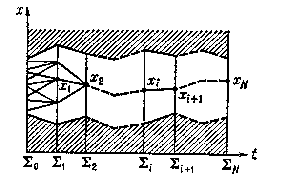
Figure: v096210a
Each family of vectors $ \{ x _ {0} \dots x _ {N} \} $ is put into correspondence with a polygon line, as shown in the figure, passing through $ x _ {0} \dots x _ {N} $ and lying in the hyperplanes $ \Sigma _ {i} $ defined by equations $ t = t _ {i} $. The length of the polygon line $ J ( x _ {0} \dots x _ {N} ) $ is the sum of the lengths $ f _ {i} ( x _ {i} , x _ {i+} 1 ) $ of its individual links. The domain of admissible $ x _ {i} $- values is defined by (17), and is separated from the forbidden domain by some polygonal line (the forbidden domain is shown shaded in the figure). The problem is to find the minimum length of a polygonal line located in the admissible domain and connecting the hyperplanes $ \Sigma _ {0} $ and $ \Sigma _ {N} $. The algorithm by which this problem is solved is a multi-step process, during which a certain set of variants $ \Omega _ {i} $ known not to contain the optimal polygonal line is marked off at each stage $ i $. The zero-th stage consists in defining the function
$$ l ( x _ {1} ) = \min _ {x _ {0} \in G _ {0} } \ f _ {0} ( x _ {0} , x _ {1} ), $$
i.e. the length of the shortest link connecting each point $ x _ {1} \in \Sigma _ {1} $ with the hyperplane $ \Sigma _ {0} $. Since
$$ \min _ {x _ {0} \in G _ {0} } J ( x _ {0} \dots x _ {N} ) = \ l ( x _ {1} ) + \sum _ {i = 1 } ^ { {N } - 1 } f _ {i} ( x _ {i} , x _ {i + 1 } ), $$
the set $ \Omega _ {0} $ of polygonal lines not containing the segment $ l( x _ {1} ) $ may be discarded. In the first stage one constructs the shortest polygonal line
$$ l ( x _ {2} ) = \ \min _ {x _ {1} \in G _ {1} } \ ( l ( x _ {1} ) + f _ {1} ( x _ {1} , x _ {2} ) ), $$
connecting each point $ x _ {2} \in \Sigma _ {2} $ with $ \Sigma _ {0} $, and the set of polygonal lines $ \Omega _ {1} $ not containing the straight line $ l( x _ {2} ) $ is also discarded, etc. In the $ i $- th stage one constructs the shortest polygonal line
$$ \tag{18 } l ( x _ {i + 1 } ) = \min _ {x _ {i} \in G _ {i} } \ ( l ( x _ {i} ) + f _ {i} ( x _ {i} , x _ {i + 1 } ) ), $$
connecting each point $ x _ {i+} 1 \in \Sigma _ {i+} 1 $ with $ \Sigma _ {0} $, and the set of polygonal lines $ \Omega _ {i} $ not containing the polygonal line $ l( x _ {i+} 1 ) $ is discarded. The last stage yields the solution of the initial problem — the shortest polygonal line connecting the hypersurfaces $ \Sigma _ {N} $ and $ \Sigma _ {0} $:
$$ l = \min _ {x _ {N} \in G _ {N} } \ l ( x _ {N} ). $$
Formula (18) is a recurrence relation which describes the multi-step process for finding the solution. It is the base of dynamic programming and of Bellman's optimality principle.
In accordance with (18), the minimum must be found on sets $ G _ {i} $ with, generally speaking, the cardinality of the continuum. The numerical realization involves a finite-dimensional approximation of them. To do this one constructs — in addition to the grid with respect to $ t $( e.g. with a constant step $ \tau $) — also a grid with respect to $ x ^ {j} $ with step $ h ^ {j} $( $ j = 1 \dots n $). The problem is then reduced to finding the shortest path in a special graph, with the grid nodes as vertices. Let $ P _ {k} ( i) $ be the node $ k $ lying in the hyperplane $ \Sigma _ {i} $; let
$$ l _ {ks} ( i) = f _ {i} ( P _ {k} ( i), P _ {s} ( i + 1)) $$
be the length of the segment connecting two nodes $ k $ and $ s $ in neighbouring hyperplanes; and let $ l _ {k} ( i) $ be the length of the shortest path connecting the node $ P _ {k} ( i) $ with the hyperplane $ \Sigma _ {0} $. The recurrence relation (18) will then assume the form
$$ l _ {s} ( i + 1) = \min _ { k } ( l _ {k} ( i) + l _ {ks} ( i) ), $$
where the minimum is taken over the numbers $ k $ of all nodes located in the admissible domain $ G _ {i} $ of the hyperplane $ \Sigma _ {i} $. In the general case this minimum is found by inspecting all nodes. This method makes it possible to find a global extremum of the function (16), subject to (3), (4) and (15), with an accuracy determined by the steps $ \tau $ and $ h ^ {j} $ of the grids. In order that the method converge to the solution of the initial problem, certain relations between these steps (e.g. of the type $ h ^ {j} = o ( \tau ) $) must hold. The method requires the use of fast computers with large memories. For this reason, the first step in practical work is to find a solution on a coarse grid, after which a finer grid is used to obtain a more exact solution in a neighbourhood of the solution thus found. This is done with the aid of one of the methods for finding a local extremum (cf. Travelling-tube method; Local variations, method of; Travelling-wave method).
References
| [1] | N.N. Moiseev, "Computational methods in the theory of optimal systems" , Moscow (1971) (In Russian) |
| [2] | L.V. Kantorovich, V.I. Krylov, "Approximate methods of higher analysis" , Noordhoff (1958) (Translated from Russian) |
| [3] | V.K. Isaev, V.V. Sonin, "Numerical aspects of the problem of optimum flight as a boundary value problem" USSR Comput. Math. Math. Phys. , 5 : 2 (1965) pp. 117–129 Zh. Vychisl. Mat. i Mat. Fiz. , 5 : 2 (1965) pp. 252–261 |
| [4] | S. Dzhurovich, D. Makintair, Raketnaya Tekhn. : 9 (1962) pp. 47–53 |
| [5] | V. Denkhem, V. Braison, Raketnaya Tekhn. i Kosmonavtika : 1 (1964) pp. 34–47 |
| [6] | L.I. Shatrovskii, "On a numerical method of solving problems of optimum control" USSR Comput. Math. Math. Phys. , 2 : 3 (1962) pp. 511–514 Zh. Vychisl. Mat. i Mat. Fiz. , 2 : 3 (1962) pp. 488–491 |
| [7] | T.M. Eneev, Kosmicheskie Issl. , 4 : 5 (1966) pp. 651–659 |
| [8] | I.A. Krylov, F.L. Chernous'ko, "On a method of successive approximations for the solution of problems of optimal control" USSR Comput. Math. Math. Phys. , 2 : 6 (1962) pp. 1371–1382 Zh. Vychisl. Mat. i Mat. Fiz. , 2 : 6 (1962) pp. 1132–1139 |
| [9] | R.P. Fedorenko, "Approximate solution of some optimal control problems" USSR Comput. Math. Math. Phys. , 4 : 6 (1964) pp. 89–116 Zh. Vychisl. Mat. i Mat. Fiz. , 4 : 6 (1964) pp. 1045–1064 |
| [10] | R. Bellman, "Dynamic programming" , Princeton Univ. Press (1957) |
| [11] | V.S. Mikhalevich, "Sequential optimization algorithms and their application. Part I" Cybernetics , 1 : 1 (1965) pp. 44–56 Kibernetika (Kiev) , 1 : 1 (1965) pp. 45–56 |
| [12] | N.N. Moiseev, "Numerical methods of optimal control theory using variations in the state space" Cybernetics , 2 : 3 (1966) pp. 1–24 Kibernetika (Kiev) , 2 : 3 (1966) pp. 1–29 |
| [13] | Yu.M. Ermol'ev, V.P. Gulenko, "The finite-difference method in optimal control problems" Cybernetics , 3 : 3 (1967) pp. 1–16 Kibernetika (Kiev) , 3 : 3 (1967) pp. 1–20 |
Comments
"Phase coordinates" are usually called "state variablestate variables" in the Western literature.
References
| [a1] | A.E. Bryson, Y.-C. Ho, "Applied optimal control" , Hemisphere (1975) |
Variational calculus, numerical methods of. Encyclopedia of Mathematics. URL: http://encyclopediaofmath.org/index.php?title=Variational_calculus,_numerical_methods_of&oldid=15104