Difference between revisions of "User:Maximilian Janisch/Sandbox"
(AUTOMATIC EDIT (latexlist): Replaced 61 formulas out of 64 by TEX code with an average confidence of 0.7943966191377944 and a minimal confidence of 0.19217438496037242.) |
(Undo revision 43847 by Maximilian Janisch (talk)) |
||
| Line 1: | Line 1: | ||
| − | + | <div class="Vorlage_Achtung" style="border: 0.18em solid #FF6666; border-left:1em solid #FF6666; margin:0.5em 0em; overflow:hidden; padding:0.5em; text-align: left;"> | |
This page is a copy of the article [[Bayesian approach]] in order to test [[User:Maximilian_Janisch/latexlist|automatic LaTeXification]]. This article is not my work. | This page is a copy of the article [[Bayesian approach]] in order to test [[User:Maximilian_Janisch/latexlist|automatic LaTeXification]]. This article is not my work. | ||
</div> | </div> | ||
| Line 5: | Line 5: | ||
''to statistical problems'' | ''to statistical problems'' | ||
| − | An approach based on the assumption that to any parameter in a statistical problem there can be assigned a definite probability distribution. Any general statistical decision problem is determined by the following elements: by a space | + | An approach based on the assumption that to any parameter in a statistical problem there can be assigned a definite probability distribution. Any general statistical decision problem is determined by the following elements: by a space <img align="absmiddle" border="0" src="https://www.encyclopediaofmath.org/legacyimages/b/b015/b015390/b0153901.png" /> of (potential) samples <img align="absmiddle" border="0" src="https://www.encyclopediaofmath.org/legacyimages/b/b015/b015390/b0153902.png" />, by a space <img align="absmiddle" border="0" src="https://www.encyclopediaofmath.org/legacyimages/b/b015/b015390/b0153903.png" /> of values of the unknown parameter <img align="absmiddle" border="0" src="https://www.encyclopediaofmath.org/legacyimages/b/b015/b015390/b0153904.png" />, by a family of probability distributions <img align="absmiddle" border="0" src="https://www.encyclopediaofmath.org/legacyimages/b/b015/b015390/b0153905.png" /> on <img align="absmiddle" border="0" src="https://www.encyclopediaofmath.org/legacyimages/b/b015/b015390/b0153906.png" />, by a space of decisions <img align="absmiddle" border="0" src="https://www.encyclopediaofmath.org/legacyimages/b/b015/b015390/b0153907.png" /> and by a function <img align="absmiddle" border="0" src="https://www.encyclopediaofmath.org/legacyimages/b/b015/b015390/b0153908.png" />, which characterizes the losses caused by accepting the decision <img align="absmiddle" border="0" src="https://www.encyclopediaofmath.org/legacyimages/b/b015/b015390/b0153909.png" /> when the true value of the parameter is <img align="absmiddle" border="0" src="https://www.encyclopediaofmath.org/legacyimages/b/b015/b015390/b01539010.png" />. The objective of decision making is to find in a certain sense an optimal rule (decision function) <img align="absmiddle" border="0" src="https://www.encyclopediaofmath.org/legacyimages/b/b015/b015390/b01539011.png" />, assigning to each result of an observation <img align="absmiddle" border="0" src="https://www.encyclopediaofmath.org/legacyimages/b/b015/b015390/b01539012.png" /> the decision <img align="absmiddle" border="0" src="https://www.encyclopediaofmath.org/legacyimages/b/b015/b015390/b01539013.png" />. In the Bayesian approach, when it is assumed that the unknown parameter <img align="absmiddle" border="0" src="https://www.encyclopediaofmath.org/legacyimages/b/b015/b015390/b01539014.png" /> is a random variable with a given (a priori) distribution <img align="absmiddle" border="0" src="https://www.encyclopediaofmath.org/legacyimages/b/b015/b015390/b01539015.png" /> on <img align="absmiddle" border="0" src="https://www.encyclopediaofmath.org/legacyimages/b/b015/b015390/b01539016.png" /> the best decision function ([[Bayesian decision function|Bayesian decision function]]) <img align="absmiddle" border="0" src="https://www.encyclopediaofmath.org/legacyimages/b/b015/b015390/b01539017.png" /> is defined as the function for which the minimum expected loss <img align="absmiddle" border="0" src="https://www.encyclopediaofmath.org/legacyimages/b/b015/b015390/b01539018.png" />, where |
| − | + | <table class="eq" style="width:100%;"> <tr><td valign="top" style="width:94%;text-align:center;"><img align="absmiddle" border="0" src="https://www.encyclopediaofmath.org/legacyimages/b/b015/b015390/b01539019.png" /></td> </tr></table> | |
and | and | ||
| − | + | <table class="eq" style="width:100%;"> <tr><td valign="top" style="width:94%;text-align:center;"><img align="absmiddle" border="0" src="https://www.encyclopediaofmath.org/legacyimages/b/b015/b015390/b01539020.png" /></td> </tr></table> | |
is attained. Thus, | is attained. Thus, | ||
| − | + | <table class="eq" style="width:100%;"> <tr><td valign="top" style="width:94%;text-align:center;"><img align="absmiddle" border="0" src="https://www.encyclopediaofmath.org/legacyimages/b/b015/b015390/b01539021.png" /></td> </tr></table> | |
| − | In searching for the Bayesian decision function | + | In searching for the Bayesian decision function <img align="absmiddle" border="0" src="https://www.encyclopediaofmath.org/legacyimages/b/b015/b015390/b01539022.png" />, the following remark is useful. Let <img align="absmiddle" border="0" src="https://www.encyclopediaofmath.org/legacyimages/b/b015/b015390/b01539023.png" />, <img align="absmiddle" border="0" src="https://www.encyclopediaofmath.org/legacyimages/b/b015/b015390/b01539024.png" />, where <img align="absmiddle" border="0" src="https://www.encyclopediaofmath.org/legacyimages/b/b015/b015390/b01539025.png" /> and <img align="absmiddle" border="0" src="https://www.encyclopediaofmath.org/legacyimages/b/b015/b015390/b01539026.png" /> are certain <img align="absmiddle" border="0" src="https://www.encyclopediaofmath.org/legacyimages/b/b015/b015390/b01539027.png" />-finite measures. One then finds, assuming that the order of integration may be changed, |
| − | + | <table class="eq" style="width:100%;"> <tr><td valign="top" style="width:94%;text-align:center;"><img align="absmiddle" border="0" src="https://www.encyclopediaofmath.org/legacyimages/b/b015/b015390/b01539028.png" /></td> </tr></table> | |
| − | + | <table class="eq" style="width:100%;"> <tr><td valign="top" style="width:94%;text-align:center;"><img align="absmiddle" border="0" src="https://www.encyclopediaofmath.org/legacyimages/b/b015/b015390/b01539029.png" /></td> </tr></table> | |
| − | + | <table class="eq" style="width:100%;"> <tr><td valign="top" style="width:94%;text-align:center;"><img align="absmiddle" border="0" src="https://www.encyclopediaofmath.org/legacyimages/b/b015/b015390/b01539030.png" /></td> </tr></table> | |
| − | It is seen from the above that for a given | + | It is seen from the above that for a given <img align="absmiddle" border="0" src="https://www.encyclopediaofmath.org/legacyimages/b/b015/b015390/b01539031.png" /> is that value of <img align="absmiddle" border="0" src="https://www.encyclopediaofmath.org/legacyimages/b/b015/b015390/b01539032.png" /> for which |
| − | <table class="eq" style="width:100%;" | + | <table class="eq" style="width:100%;"> <tr><td valign="top" style="width:94%;text-align:center;"><img align="absmiddle" border="0" src="https://www.encyclopediaofmath.org/legacyimages/b/b015/b015390/b01539033.png" /></td> </tr></table> |
is attained, or, what is equivalent, for which | is attained, or, what is equivalent, for which | ||
| − | + | <table class="eq" style="width:100%;"> <tr><td valign="top" style="width:94%;text-align:center;"><img align="absmiddle" border="0" src="https://www.encyclopediaofmath.org/legacyimages/b/b015/b015390/b01539034.png" /></td> </tr></table> | |
is attained, where | is attained, where | ||
| − | + | <table class="eq" style="width:100%;"> <tr><td valign="top" style="width:94%;text-align:center;"><img align="absmiddle" border="0" src="https://www.encyclopediaofmath.org/legacyimages/b/b015/b015390/b01539035.png" /></td> </tr></table> | |
But, according to the [[Bayes formula|Bayes formula]] | But, according to the [[Bayes formula|Bayes formula]] | ||
| − | + | <table class="eq" style="width:100%;"> <tr><td valign="top" style="width:94%;text-align:center;"><img align="absmiddle" border="0" src="https://www.encyclopediaofmath.org/legacyimages/b/b015/b015390/b01539036.png" /></td> </tr></table> | |
| − | Thus, for a given | + | Thus, for a given <img align="absmiddle" border="0" src="https://www.encyclopediaofmath.org/legacyimages/b/b015/b015390/b01539037.png" />, <img align="absmiddle" border="0" src="https://www.encyclopediaofmath.org/legacyimages/b/b015/b015390/b01539038.png" /> is that value of <img align="absmiddle" border="0" src="https://www.encyclopediaofmath.org/legacyimages/b/b015/b015390/b01539039.png" /> for which the conditional average loss <img align="absmiddle" border="0" src="https://www.encyclopediaofmath.org/legacyimages/b/b015/b015390/b01539040.png" /> attains a minimum. |
| − | Example. (The Bayesian approach applied to the case of distinguishing between two simple hypotheses.) Let | + | Example. (The Bayesian approach applied to the case of distinguishing between two simple hypotheses.) Let <img align="absmiddle" border="0" src="https://www.encyclopediaofmath.org/legacyimages/b/b015/b015390/b01539041.png" />, <img align="absmiddle" border="0" src="https://www.encyclopediaofmath.org/legacyimages/b/b015/b015390/b01539042.png" />, <img align="absmiddle" border="0" src="https://www.encyclopediaofmath.org/legacyimages/b/b015/b015390/b01539043.png" />, <img align="absmiddle" border="0" src="https://www.encyclopediaofmath.org/legacyimages/b/b015/b015390/b01539044.png" />; <img align="absmiddle" border="0" src="https://www.encyclopediaofmath.org/legacyimages/b/b015/b015390/b01539045.png" />, <img align="absmiddle" border="0" src="https://www.encyclopediaofmath.org/legacyimages/b/b015/b015390/b01539046.png" />, <img align="absmiddle" border="0" src="https://www.encyclopediaofmath.org/legacyimages/b/b015/b015390/b01539047.png" />. If the solution <img align="absmiddle" border="0" src="https://www.encyclopediaofmath.org/legacyimages/b/b015/b015390/b01539048.png" /> is identified with the acceptance of the hypothesis <img align="absmiddle" border="0" src="https://www.encyclopediaofmath.org/legacyimages/b/b015/b015390/b01539049.png" />: <img align="absmiddle" border="0" src="https://www.encyclopediaofmath.org/legacyimages/b/b015/b015390/b01539050.png" />, it is natural to assume that <img align="absmiddle" border="0" src="https://www.encyclopediaofmath.org/legacyimages/b/b015/b015390/b01539051.png" />, <img align="absmiddle" border="0" src="https://www.encyclopediaofmath.org/legacyimages/b/b015/b015390/b01539052.png" />. Then |
| − | + | <table class="eq" style="width:100%;"> <tr><td valign="top" style="widtutomatic LaTeXificationh:94%;text-align:center;"><img align="absmiddle" border="0" src="https://www.encyclopediaofmath.org/legacyimages/b/b015/b015390/b01539053.png" /></td> </tr></table> | |
| − | + | <table class="eq" style="width:100%;"> <tr><td valign="top" style="width:94%;text-align:center;"><img align="absmiddle" border="0" src="https://www.encyclopediaofmath.org/legacyimages/b/b015/b015390/b01539054.png" /></td> </tr></table> | |
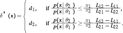
| − | implies that | + | implies that <img align="absmiddle" border="0" src="https://www.encyclopediaofmath.org/legacyimages/b/b015/b015390/b01539055.png" /> is attained for the function |
| − | + | <table class="eq" style="width:100%;"> <tr><td valign="top" style="width:94%;text-align:center;"><img align="absmiddle" border="0" src="https://www.encyclopediaofmath.org/legacyimages/b/b015/b015390/b01539056.png" /></td> </tr></table> | |
| − | The advantage of the Bayesian approach consists in the fact that, unlike the losses | + | The advantage of the Bayesian approach consists in the fact that, unlike the losses <img align="absmiddle" border="0" src="https://www.encyclopediaofmath.org/legacyimages/b/b015/b015390/b01539057.png" />, the expected losses <img align="absmiddle" border="0" src="https://www.encyclopediaofmath.org/legacyimages/b/b015/b015390/b01539058.png" /> are numbers which are dependent on the unknown parameter <img align="absmiddle" border="0" src="https://www.encyclopediaofmath.org/legacyimages/b/b015/b015390/b01539059.png" />, and, consequently, it is known that solutions <img align="absmiddle" border="0" src="https://www.encyclopediaofmath.org/legacyimages/b/b015/b015390/b01539060.png" /> for which |
| − | + | <table class="eq" style="width:100%;"> <tr><td valign="top" style="width:94%;text-align:center;"><img align="absmiddle" border="0" src="https://www.encyclopediaofmath.org/legacyimages/b/b015/b015390/b01539061.png" /></td> </tr></table> | |
| − | and which are, if not optimal, at least <img align="absmiddle" border="0" src="https://www.encyclopediaofmath.org/legacyimages/b/b015/b015390/b01539062.png"/>-optimal | + | and which are, if not optimal, at least <img align="absmiddle" border="0" src="https://www.encyclopediaofmath.org/legacyimages/b/b015/b015390/b01539062.png" />-optimal <img align="absmiddle" border="0" src="https://www.encyclopediaofmath.org/legacyimages/b/b015/b015390/b01539063.png" />, are certain to exist. The disadvantage of the Bayesian approach is the necessity of postulating both the existence of an a priori distribution of the unknown parameter and its precise form (the latter disadvantage may be overcome to a certain extent by adopting an empirical Bayesian approach, cf. [[Bayesian approach, empirical|Bayesian approach, empirical]]). |
====References==== | ====References==== | ||
| − | <table>< | + | <table><TR><TD valign="top">[1]</TD> <TD valign="top"> A. Wald, "Statistical decision functions" , Wiley (1950)</TD></TR><TR><TD valign="top">[2]</TD> <TD valign="top"> M.H. de Groot, "Optimal statistical decisions" , McGraw-Hill (1970)</TD></TR></table> |
Revision as of 22:01, 1 September 2019
to statistical problems
An approach based on the assumption that to any parameter in a statistical problem there can be assigned a definite probability distribution. Any general statistical decision problem is determined by the following elements: by a space  of (potential) samples
  , by a space
  of values of the unknown parameter
  , by a family of probability distributions
  on
on  , by a space of decisions
  and by a function
  , which characterizes the losses caused by accepting the decision
  when the true value of the parameter is
  . The objective of decision making is to find in a certain sense an optimal rule (decision function)
  , assigning to each result of an observation
  the decision
  . In the Bayesian approach, when it is assumed that the unknown parameter
  is a random variable with a given (a priori) distribution
  on
on  the best decision function (Bayesian decision function)
  is defined as the function for which the minimum expected loss
 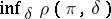 , where
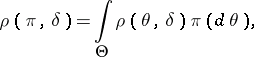 |
and
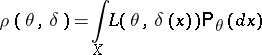 |
is attained. Thus,
 |
In searching for the Bayesian decision function  , the following remark is useful. Let
  ,
,  , where
  and
and  are certain
  -finite measures. One then finds, assuming that the order of integration may be changed,
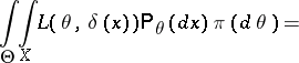 |
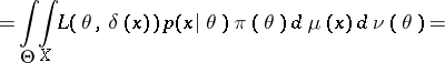 |
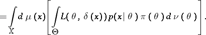 |
It is seen from the above that for a given  is that value of
  for which
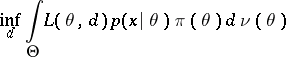 |
is attained, or, what is equivalent, for which
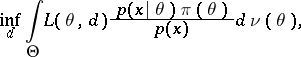 |
is attained, where
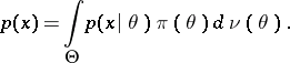 |
But, according to the Bayes formula
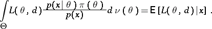 |
Thus, for a given  ,
,  is that value of
  for which the conditional average loss
  attains a minimum.
Example. (The Bayesian approach applied to the case of distinguishing between two simple hypotheses.) Let  ,
,  ,
,  ,
,  ;
;  ,
,  ,
,  . If the solution
  is identified with the acceptance of the hypothesis
  :
:  , it is natural to assume that
  ,
,  . Then
 |
 |
implies that  is attained for the function
 |
The advantage of the Bayesian approach consists in the fact that, unlike the losses  , the expected losses
  are numbers which are dependent on the unknown parameter
  , and, consequently, it is known that solutions
  for which
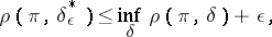 |
and which are, if not optimal, at least  -optimal
  , are certain to exist. The disadvantage of the Bayesian approach is the necessity of postulating both the existence of an a priori distribution of the unknown parameter and its precise form (the latter disadvantage may be overcome to a certain extent by adopting an empirical Bayesian approach, cf. Bayesian approach, empirical).
References
| [1] | A. Wald, "Statistical decision functions" , Wiley (1950) |
| [2] | M.H. de Groot, "Optimal statistical decisions" , McGraw-Hill (1970) |
Maximilian Janisch/Sandbox. Encyclopedia of Mathematics. URL: http://encyclopediaofmath.org/index.php?title=Maximilian_Janisch/Sandbox&oldid=43848