Difference between revisions of "User:Maximilian Janisch/Sandbox"
(copy of fourier transform article) |
(AUTOMATIC EDIT (Latexlist): Replaced 18.2% images by TEX code) |
||
| Line 1: | Line 1: | ||
| − | {{TEX|part}} | + | {{TEX|partial}}{{TEX|part}} |
One of the integral transforms (cf. [[Integral transform|Integral transform]]). It is a linear operator $F$ acting on a space whose elements are functions $f$ of $n$ real variables. The smallest domain of definition of $F$ is the set $D=C_0^\infty$ of all infinitely-differentiable functions $\phi$ of compact support. For such functions | One of the integral transforms (cf. [[Integral transform|Integral transform]]). It is a linear operator $F$ acting on a space whose elements are functions $f$ of $n$ real variables. The smallest domain of definition of $F$ is the set $D=C_0^\infty$ of all infinitely-differentiable functions $\phi$ of compact support. For such functions | ||
| Line 11: | Line 11: | ||
Formula (1) also acts on the space $L_{1}\left(\mathbf{R}^{n}\right)$ of integrable functions. In order to enlarge the domain of definition of the operator $F$ generalization of (1) is necessary. In classical analysis such a generalization has been constructed for locally integrable functions with some restriction on their behaviour as $|x|\to\infty$ (see [[Fourier integral|Fourier integral]]). In the theory of generalized functions the definition of the operator $F$ is free of many requirements of classical analysis. | Formula (1) also acts on the space $L_{1}\left(\mathbf{R}^{n}\right)$ of integrable functions. In order to enlarge the domain of definition of the operator $F$ generalization of (1) is necessary. In classical analysis such a generalization has been constructed for locally integrable functions with some restriction on their behaviour as $|x|\to\infty$ (see [[Fourier integral|Fourier integral]]). In the theory of generalized functions the definition of the operator $F$ is free of many requirements of classical analysis. | ||
| − | The basic problems connected with the study of the Fourier transform $F$ are: the investigation of the domain of definition <img align="absmiddle" border="0" src="https://www.encyclopediaofmath.org/legacyimages/f/f041/f041150/f04115023.png" /> and the range of values <img align="absmiddle" border="0" src="https://www.encyclopediaofmath.org/legacyimages/f/f041/f041150/f04115024.png" /> of <img align="absmiddle" border="0" src="https://www.encyclopediaofmath.org/legacyimages/f/f041/f041150/f04115025.png" />; as well as studying properties of the mapping | + | The basic problems connected with the study of the Fourier transform $F$ are: the investigation of the domain of definition <img align="absmiddle" border="0" src="https://www.encyclopediaofmath.org/legacyimages/f/f041/f041150/f04115023.png"/> and the range of values <img align="absmiddle" border="0" src="https://www.encyclopediaofmath.org/legacyimages/f/f041/f041150/f04115024.png"/> of <img align="absmiddle" border="0" src="https://www.encyclopediaofmath.org/legacyimages/f/f041/f041150/f04115025.png"/>; as well as studying properties of the mapping $\Phi \rightarrow \Psi$ (in particular, conditions for the existence of the inverse operator <img align="absmiddle" border="0" src="https://www.encyclopediaofmath.org/legacyimages/f/f041/f041150/f04115027.png"/> and its expression). The inversion formula for the Fourier transform is very simple: |
| − | <table class="eq" style="width:100%;"> <tr><td | + | <table class="eq" style="width:100%;"> <tbody><tr><td style="width:94%;text-align:center;" valign="top"><img align="absmiddle" border="0" src="https://www.encyclopediaofmath.org/legacyimages/f/f041/f041150/f04115028.png"/></td> </tr></tbody></table> |
| − | Under the action of the Fourier transform linear operators on the original space, which are invariant with respect to a shift, become (under certain conditions) multiplication operators in the image space. In particular, the convolution of two functions <img align="absmiddle" border="0" src="https://www.encyclopediaofmath.org/legacyimages/f/f041/f041150/f04115029.png" /> and <img align="absmiddle" border="0" src="https://www.encyclopediaofmath.org/legacyimages/f/f041/f041150/f04115030.png" /> goes over into the product of the functions <img align="absmiddle" border="0" src="https://www.encyclopediaofmath.org/legacyimages/f/f041/f041150/f04115031.png" /> and <img align="absmiddle" border="0" src="https://www.encyclopediaofmath.org/legacyimages/f/f041/f041150/f04115032.png" />: | + | Under the action of the Fourier transform linear operators on the original space, which are invariant with respect to a shift, become (under certain conditions) multiplication operators in the image space. In particular, the convolution of two functions <img align="absmiddle" border="0" src="https://www.encyclopediaofmath.org/legacyimages/f/f041/f041150/f04115029.png"/> and <img align="absmiddle" border="0" src="https://www.encyclopediaofmath.org/legacyimages/f/f041/f041150/f04115030.png"/> goes over into the product of the functions <img align="absmiddle" border="0" src="https://www.encyclopediaofmath.org/legacyimages/f/f041/f041150/f04115031.png"/> and <img align="absmiddle" border="0" src="https://www.encyclopediaofmath.org/legacyimages/f/f041/f041150/f04115032.png"/>: |
| − | <table class="eq" style="width:100%;"> <tr><td | + | <table class="eq" style="width:100%;"> <tbody><tr><td style="width:94%;text-align:center;" valign="top"><img align="absmiddle" border="0" src="https://www.encyclopediaofmath.org/legacyimages/f/f041/f041150/f04115033.png"/></td> </tr></tbody></table> |
and differentiation induces multiplication by the independent variable: | and differentiation induces multiplication by the independent variable: | ||
| − | + | \begin{equation} F ( D ^ { \alpha } f ) = ( i x ) ^ { \alpha } F f \end{equation} | |
| − | In the spaces | + | In the spaces $L _ { p } ( R ^ { n } )$, <img align="absmiddle" border="0" src="https://www.encyclopediaofmath.org/legacyimages/f/f041/f041150/f04115036.png"/>, the operator <img align="absmiddle" border="0" src="https://www.encyclopediaofmath.org/legacyimages/f/f041/f041150/f04115037.png"/> is defined by the formula (1) on the set <img align="absmiddle" border="0" src="https://www.encyclopediaofmath.org/legacyimages/f/f041/f041150/f04115038.png"/> and is a bounded operator from $L _ { p } ( R ^ { n } )$ into <img align="absmiddle" border="0" src="https://www.encyclopediaofmath.org/legacyimages/f/f041/f041150/f04115040.png"/>, $p ^ { - 1 } + q ^ { - 1 } = 1$: |
\begin{equation} \left\{\frac{1}{(2 \pi)^{n / 2}} \int_{\mathbf{R}^{n}}|(F f)(x)|^{q} d x\right\}^{1 / q} \leq\left\{\frac{1}{(2 \pi)^{n / 2}} \int_{\mathbf{R}^{n}}|f(x)|^{p} d x\right\}^{1 / p} \end{equation} | \begin{equation} \left\{\frac{1}{(2 \pi)^{n / 2}} \int_{\mathbf{R}^{n}}|(F f)(x)|^{q} d x\right\}^{1 / q} \leq\left\{\frac{1}{(2 \pi)^{n / 2}} \int_{\mathbf{R}^{n}}|f(x)|^{p} d x\right\}^{1 / p} \end{equation} | ||
| − | (the Hausdorff–Young inequality). <img align="absmiddle" border="0" src="https://www.encyclopediaofmath.org/legacyimages/f/f041/f041150/f04115043.png" /> admits a continuous extension onto the whole space <img align="absmiddle" border="0" src="https://www.encyclopediaofmath.org/legacyimages/f/f041/f041150/f04115044.png" /> which (for | + | (the Hausdorff–Young inequality). <img align="absmiddle" border="0" src="https://www.encyclopediaofmath.org/legacyimages/f/f041/f041150/f04115043.png"/> admits a continuous extension onto the whole space <img align="absmiddle" border="0" src="https://www.encyclopediaofmath.org/legacyimages/f/f041/f041150/f04115044.png"/> which (for $1 < p \leq 2$) is given by |
| − | <table class="eq" style="width:100%;"> <tr><td | + | <table class="eq" style="width:100%;"> <tbody><tr><td style="width:94%;text-align:center;" valign="top"><img align="absmiddle" border="0" src="https://www.encyclopediaofmath.org/legacyimages/f/f041/f041150/f04115046.png"/></td> <td style="width:5%;text-align:right;" valign="top">(3)</td></tr></tbody></table> |
| − | Convergence is understood to be in the norm of <img align="absmiddle" border="0" src="https://www.encyclopediaofmath.org/legacyimages/f/f041/f041150/f04115047.png" />. If | + | Convergence is understood to be in the norm of <img align="absmiddle" border="0" src="https://www.encyclopediaofmath.org/legacyimages/f/f041/f041150/f04115047.png"/>. If $p \neq 2$, the image of <img align="absmiddle" border="0" src="https://www.encyclopediaofmath.org/legacyimages/f/f041/f041150/f04115049.png"/> under the action of <img align="absmiddle" border="0" src="https://www.encyclopediaofmath.org/legacyimages/f/f041/f041150/f04115050.png"/> does not coincide with <img align="absmiddle" border="0" src="https://www.encyclopediaofmath.org/legacyimages/f/f041/f041150/f04115051.png"/>, that is, the imbedding <img align="absmiddle" border="0" src="https://www.encyclopediaofmath.org/legacyimages/f/f041/f041150/f04115052.png"/> is strict when <img align="absmiddle" border="0" src="https://www.encyclopediaofmath.org/legacyimages/f/f041/f041150/f04115053.png"/> (for the case <img align="absmiddle" border="0" src="https://www.encyclopediaofmath.org/legacyimages/f/f041/f041150/f04115054.png"/> see [[Plancherel theorem|Plancherel theorem]]). The inverse operator <img align="absmiddle" border="0" src="https://www.encyclopediaofmath.org/legacyimages/f/f041/f041150/f04115055.png"/> is defined on $F L y$ by |
| − | <table class="eq" style="width:100%;"> <tr><td | + | <table class="eq" style="width:100%;"> <tbody><tr><td style="width:94%;text-align:center;" valign="top"><img align="absmiddle" border="0" src="https://www.encyclopediaofmath.org/legacyimages/f/f041/f041150/f04115057.png"/></td> </tr></tbody></table> |
The problem of extending the Fourier transform to a larger class of functions arises constantly in analysis and its applications. See, for example, [[Fourier transform of a generalized function|Fourier transform of a generalized function]]. | The problem of extending the Fourier transform to a larger class of functions arises constantly in analysis and its applications. See, for example, [[Fourier transform of a generalized function|Fourier transform of a generalized function]]. | ||
====References==== | ====References==== | ||
| − | <table>< | + | <table><tbody><tr><td valign="top">[1]</td> <td valign="top"> E.C. Titchmarsh, "Introduction to the theory of Fourier integrals" , Oxford Univ. Press (1948)</td></tr><tr><td valign="top">[2]</td> <td valign="top"> A. Zygmund, "Trigonometric series" , '''2''' , Cambridge Univ. Press (1988)</td></tr><tr><td valign="top">[3]</td> <td valign="top"> E.M. Stein, G. Weiss, "Fourier analysis on Euclidean spaces" , Princeton Univ. Press (1971)</td></tr></tbody></table> |
| Line 45: | Line 45: | ||
Instead of "generalized function" the term "distributiondistribution" is often used. | Instead of "generalized function" the term "distributiondistribution" is often used. | ||
| − | If <img align="absmiddle" border="0" src="https://www.encyclopediaofmath.org/legacyimages/f/f041/f041150/f04115058.png" /> and <img align="absmiddle" border="0" src="https://www.encyclopediaofmath.org/legacyimages/f/f041/f041150/f04115059.png" /> then <img align="absmiddle" border="0" src="https://www.encyclopediaofmath.org/legacyimages/f/f041/f041150/f04115060.png" /> denotes the scalar product <img align="absmiddle" border="0" src="https://www.encyclopediaofmath.org/legacyimages/f/f041/f041150/f04115061.png" />. | + | If <img align="absmiddle" border="0" src="https://www.encyclopediaofmath.org/legacyimages/f/f041/f041150/f04115058.png"/> and <img align="absmiddle" border="0" src="https://www.encyclopediaofmath.org/legacyimages/f/f041/f041150/f04115059.png"/> then <img align="absmiddle" border="0" src="https://www.encyclopediaofmath.org/legacyimages/f/f041/f041150/f04115060.png"/> denotes the scalar product <img align="absmiddle" border="0" src="https://www.encyclopediaofmath.org/legacyimages/f/f041/f041150/f04115061.png"/>. |
| − | If in (1) the "normalizing factor" | + | If in (1) the "normalizing factor" $( 1 / 2 \pi ) ^ { n / 2 }$ is replaced by some constant <img align="absmiddle" border="0" src="https://www.encyclopediaofmath.org/legacyimages/f/f041/f041150/f04115063.png"/>, then in (2) it must be replaced by <img align="absmiddle" border="0" src="https://www.encyclopediaofmath.org/legacyimages/f/f041/f041150/f04115064.png"/> with $\beta = ( 1 / 2 \pi ) ^ { x }$. |
At least two other conventions for the "normalization factor" are in common use: | At least two other conventions for the "normalization factor" are in common use: | ||
| − | <table class="eq" style="width:100%;"> <tr><td | + | <table class="eq" style="width:100%;"> <tbody><tr><td style="width:94%;text-align:center;" valign="top"><img align="absmiddle" border="0" src="https://www.encyclopediaofmath.org/legacyimages/f/f041/f041150/f04115066.png"/></td> <td style="width:5%;text-align:right;" valign="top">(a1)</td></tr></tbody></table> |
| − | <table class="eq" style="width:100%;"> <tr><td | + | <table class="eq" style="width:100%;"> <tbody><tr><td style="width:94%;text-align:center;" valign="top"><img align="absmiddle" border="0" src="https://www.encyclopediaofmath.org/legacyimages/f/f041/f041150/f04115067.png"/></td> </tr></tbody></table> |
| − | <table class="eq" style="width:100%;"> <tr><td | + | <table class="eq" style="width:100%;"> <tbody><tr><td style="width:94%;text-align:center;" valign="top"><img align="absmiddle" border="0" src="https://www.encyclopediaofmath.org/legacyimages/f/f041/f041150/f04115068.png"/></td> <td style="width:5%;text-align:right;" valign="top">(a2)</td></tr></tbody></table> |
| − | <table class="eq" style="width:100%;"> <tr><td | + | <table class="eq" style="width:100%;"> <tbody><tr><td style="width:94%;text-align:center;" valign="top"><img align="absmiddle" border="0" src="https://www.encyclopediaofmath.org/legacyimages/f/f041/f041150/f04115069.png"/></td> </tr></tbody></table> |
| − | The convention of the article leads to the Fourier transform as a [[Unitary operator|unitary operator]] from <img align="absmiddle" border="0" src="https://www.encyclopediaofmath.org/legacyimages/f/f041/f041150/f04115070.png" /> into itself, and so does the convention (a2). Convention (a1) is more in line with [[Harmonic analysis|harmonic analysis]]. | + | The convention of the article leads to the Fourier transform as a [[Unitary operator|unitary operator]] from <img align="absmiddle" border="0" src="https://www.encyclopediaofmath.org/legacyimages/f/f041/f041150/f04115070.png"/> into itself, and so does the convention (a2). Convention (a1) is more in line with [[Harmonic analysis|harmonic analysis]]. |
====References==== | ====References==== | ||
| − | <table>< | + | <table><tbody><tr><td valign="top">[a1]</td> <td valign="top"> W. Rudin, "Functional analysis" , McGraw-Hill (1973)</td></tr></tbody></table |
Revision as of 17:00, 6 April 2019
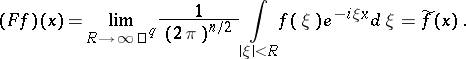
One of the integral transforms (cf. Integral transform). It is a linear operator $F$ acting on a space whose elements are functions $f$ of $n$ real variables. The smallest domain of definition of $F$ is the set $D=C_0^\infty$ of all infinitely-differentiable functions $\phi$ of compact support. For such functions
\begin{equation} (F\phi)(x) = \frac{1}{(2\pi)^{\frac{n}{2}}} \cdot \int_{\mathbf R^n} \phi(\xi) e^{-i x \xi} \, \mathrm d\xi. \end{equation}
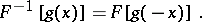
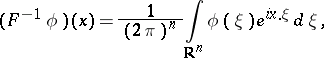
In a certain sense the most natural domain of definition of $F$ is the set $S$ of all infinitely-differentiable functions $\phi$ that, together with their derivatives, vanish at infinity faster than any power of $\frac{1}{|x|}$. Formula (1) still holds for $\phi\in S$, and $(F \phi)(x) \equiv \psi(x)\in S$. Moreover, $F$ is an isomorphism of $S$ onto itself, the inverse mapping $F^{-1}$ (the inverse Fourier transform) is the inverse of the Fourier transform and is given by the formula:
\begin{equation} \phi(x) = (F^{-1} \psi)(x) = \frac{1}{(2\pi)^{\frac{n}{2}}} \cdot \int_{\mathbf R^n} \psi(\xi) e^{i x \xi} \, \mathrm d\xi. \end{equation}
Formula (1) also acts on the space $L_{1}\left(\mathbf{R}^{n}\right)$ of integrable functions. In order to enlarge the domain of definition of the operator $F$ generalization of (1) is necessary. In classical analysis such a generalization has been constructed for locally integrable functions with some restriction on their behaviour as $|x|\to\infty$ (see Fourier integral). In the theory of generalized functions the definition of the operator $F$ is free of many requirements of classical analysis.
The basic problems connected with the study of the Fourier transform $F$ are: the investigation of the domain of definition  and the range of values
  of
of  ; as well as studying properties of the mapping $\Phi \rightarrow \Psi$ (in particular, conditions for the existence of the inverse operator
  and its expression). The inversion formula for the Fourier transform is very simple:
 |
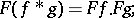
Under the action of the Fourier transform linear operators on the original space, which are invariant with respect to a shift, become (under certain conditions) multiplication operators in the image space. In particular, the convolution of two functions  and
and  goes over into the product of the functions
  and
and  :
:
 |
and differentiation induces multiplication by the independent variable:
\begin{equation} F ( D ^ { \alpha } f ) = ( i x ) ^ { \alpha } F f \end{equation}
In the spaces $L _ { p } ( R ^ { n } )$,  , the operator
  is defined by the formula (1) on the set
 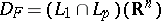 and is a bounded operator from $L _ { p } ( R ^ { n } )$ into
  , $p ^ { - 1 } + q ^ { - 1 } = 1$:
\begin{equation} \left\{\frac{1}{(2 \pi)^{n / 2}} \int_{\mathbf{R}^{n}}|(F f)(x)|^{q} d x\right\}^{1 / q} \leq\left\{\frac{1}{(2 \pi)^{n / 2}} \int_{\mathbf{R}^{n}}|f(x)|^{p} d x\right\}^{1 / p} \end{equation}
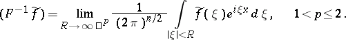
(the Hausdorff–Young inequality).  admits a continuous extension onto the whole space
  which (for $1 < p \leq 2$) is given by
 | (3) |
Convergence is understood to be in the norm of  . If $p \neq 2$, the image of
  under the action of
  does not coincide with
  , that is, the imbedding
  is strict when
  (for the case
  see Plancherel theorem). The inverse operator
  is defined on $F L y$ by
 |
The problem of extending the Fourier transform to a larger class of functions arises constantly in analysis and its applications. See, for example, Fourier transform of a generalized function.
References
<tbody></tbody>| [1] | E.C. Titchmarsh, "Introduction to the theory of Fourier integrals" , Oxford Univ. Press (1948) |
| [2] | A. Zygmund, "Trigonometric series" , 2 , Cambridge Univ. Press (1988) |
| [3] | E.M. Stein, G. Weiss, "Fourier analysis on Euclidean spaces" , Princeton Univ. Press (1971) |
Comments
Instead of "generalized function" the term "distributiondistribution" is often used.
If  and
and  then
then  denotes the scalar product
  .
.
If in (1) the "normalizing factor" $( 1 / 2 \pi ) ^ { n / 2 }$ is replaced by some constant  , then in (2) it must be replaced by
  with $\beta = ( 1 / 2 \pi ) ^ { x }$.
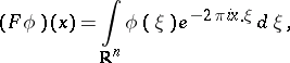
At least two other conventions for the "normalization factor" are in common use:
<tbody></tbody>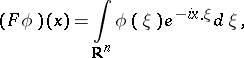 | (a1) |
 |
 | (a2) |
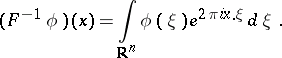 |
The convention of the article leads to the Fourier transform as a unitary operator from  into itself, and so does the convention (a2). Convention (a1) is more in line with harmonic analysis.
References
<tbody></tbody></table| [a1] | W. Rudin, "Functional analysis" , McGraw-Hill (1973) |
Maximilian Janisch/Sandbox. Encyclopedia of Mathematics. URL: http://encyclopediaofmath.org/index.php?title=Maximilian_Janisch/Sandbox&oldid=43662