Difference between revisions of "User:Boris Tsirelson/sandbox2"
(Undo revision 35590 by Boris Tsirelson (talk)) |
|||
| (179 intermediate revisions by the same user not shown) | |||
| Line 1: | Line 1: | ||
| − | + | ==Experiments== | |
| − | |||
| − | |||
| − | |||
| − | |||
| − | + | Note a fine distinction from [http://ada00.math.uni-bielefeld.de/MW1236/index.php/User:Boris_Tsirelson/sandbox#Experiments Ada]: | |
| − | + | <center><asy> | |
| − | + | fill( box((-1,-1),(1,1)), white ); | |
| − | + | draw( (-1.2,-0.5)--(1.2,-0.5) ); | |
| − | + | label("Just a text",(0,0)); | |
| − | + | filldraw( box((-0.7,-1),(0.7,1)), white, opacity(0) ); | |
| + | shipout(scale(15)*currentpicture); | ||
| + | </asy></center> | ||
| − | + | I guess, the reason is that there Asy generates pdf file (converted into png afterwards), and here something else (probably ps). | |
| − | + | No, it seems, it generates eps, both here and there. Then, what could be the reason? | |
| − | + | More. | |
| − | + | <center><asy> | |
| + | label("Just a text",(0,0)); | ||
| + | fill( box((-2,-1),(2,1)), white ); | ||
| + | //draw( box((-2,-1),(2,1)), green ); | ||
| + | shipout(scale(15)*currentpicture); | ||
| + | </asy></center> | ||
| − | |||
| − | + | <center><asy> | |
| + | label("Just a text",(0,0)); | ||
| + | fill( box((-2,-1),(2,1)), white ); | ||
| + | draw( box((-2,-1),(2,1)), green ); | ||
| + | shipout(scale(15)*currentpicture); | ||
| + | </asy></center> | ||
| − | + | Mysterious. | |
| − | + | ==Three dimensions== | |
| − | + | <center><asy> | |
| + | settings.render = 0; | ||
| − | + | unitsize(100); | |
| − | + | import three; | |
| + | import tube; | ||
| − | + | import graph; | |
| + | path unitCircle = Circle((0,0),1,35); | ||
| − | + | currentprojection = perspective((900,-350,-650)); | |
| + | currentlight=light(gray(0.4),specularfactor=3,viewport=false,(-0.5,-0.5,-0.75),(0,-0.5,0.5),(0.5,0.5,0.75)); | ||
| + | // currentlight=light(gray(0.4),specularfactor=3,viewport=false,(-0.5,-0.5,-0.75),(0.5,-0.5,0.5),(0.5,0.5,0.75)); | ||
| − | + | triple horn_start=(0,-1,0.6); | |
| + | triple horn_end=(0,0.4,0.2); | ||
| + | real horn_radius=0.2; | ||
| − | + | real ratio=horn_end.z/(-horn_start.y); // fractal levels ratio | |
| − | + | transform3 implode_right = shift(horn_end) * scale3(ratio) * rotate(-90,X) * shift(-horn_start.y*Y); | |
| + | transform3 left_right = reflect(O,X,Z)*rotate(90,Y); | ||
| − | + | path[] cover_with_holes = scale(horn_radius/ratio)*unitCircle^^ | |
| + | shift((horn_start.z,0))*scale(0.9horn_radius)*reverse(unitCircle)^^ | ||
| + | shift((-horn_start.z,0))*scale(0.9horn_radius)*reverse(unitCircle); | ||
| + | surface cover = surface(cover_with_holes,ZXplane); | ||
| + | surface cover_left = shift((horn_start.x,horn_start.y,0))*cover; | ||
| + | surface two_covers = surface(cover_left,left_right*cover_left); | ||
| − | = | + | path3 horn_axis = horn_start..horn_start+(0,0.01,0)..(0,0,0.7)..(0,0.2,0.6)..horn_end+(0,0,0.01)..horn_end; |
| − | + | surface horn = tube( horn_axis, scale(horn_radius)*unitCircle ); | |
| + | surface two_horns = surface(horn,reflect(O,X,Y)*horn); | ||
| + | surface two_horns = surface(horn,reflect(O,X,Y)*horn); | ||
| + | surface four_horns = surface(two_horns,left_right*two_horns,two_covers); | ||
| − | == | + | surface four_small_horns = implode_right*four_horns; |
| + | surface eight_small_horns = surface(four_small_horns,left_right*four_small_horns); | ||
| − | { | + | surface big_surface = surface(four_horns,eight_small_horns); |
| − | + | ||
| − | + | real R = horn_radius/ratio; | |
| − | + | ||
| − | + | draw ( circle((0,1,0), 1.005R, Y ), currentpen+2 ); | |
| − | + | draw ( circle((horn_start.z,1.01,horn_start.x), horn_radius, Y ), currentpen+2 ); | |
| − | + | draw ( circle((-horn_start.z,1.01,horn_start.x), horn_radius, Y ), currentpen+2 ); | |
| − | + | ||
| − | + | draw (big_surface, yellow); | |
| − | + | ||
| − | + | pen blackpen = currentpen+1.5; | |
| − | + | ||
| − | + | draw ( circle((0,-1,0), 1.005R, Y ), blackpen ); | |
| − | + | draw ( circle(horn_start, 0.98horn_radius, Y ), blackpen ); | |
| − | + | draw ( circle((horn_start.x,horn_start.y,-horn_start.z), 0.98horn_radius, Y ), blackpen ); | |
| − | + | ||
| − | + | real phi=0.9; // adjust to the projection | |
| − | + | triple u = (cos(phi),0,sin(phi)); | |
| − | + | draw( R*u-Y -- R*u+Y, blackpen ); | |
| + | draw( -R*u-Y -- -R*u+Y, blackpen ); | ||
| + | |||
| + | </asy></center> | ||
| + | |||
| + | |||
| + | <center><asy> | ||
| + | settings.render = 0; | ||
| + | |||
| + | size(200); | ||
| + | import graph3; | ||
| + | |||
| + | currentprojection=perspective((2,2,5)); | ||
| + | |||
| + | real R=1; | ||
| + | real a=1; | ||
| + | |||
| + | real co=0.6; | ||
| + | real colo=0.3; | ||
| + | |||
| + | triple f(pair t) { | ||
| + | return ((R+a*cos(t.y))*cos(t.x),(R+a*cos(t.y))*sin(t.x),a*sin(t.y)); | ||
| + | } | ||
| + | |||
| + | surface s=surface(f,(0,0),(2pi,2pi),20,20,Spline); | ||
| + | |||
| + | draw(s,rgb(co,co,co),meshpen=rgb(colo,colo,colo)); | ||
| + | |||
| + | </asy></center> | ||
| + | |||
| + | ==Sinusoid== | ||
| + | |||
| + | <center><asy> | ||
| + | import graph; | ||
| + | size(450); | ||
| + | real f(real x) {return sin(x);}; | ||
| + | |||
| + | real f1(real x) {return cos(x);}; | ||
| + | draw(graph(f1,-2*pi,2*pi),blue+1,"$\cos(x)$"); | ||
| + | draw(graph(f,-2*pi,2*pi),red+1,"$\sin(x)$"); | ||
| + | xaxis("$x$",Arrow); | ||
| + | yaxis(); | ||
| + | |||
| + | xtick("$\frac{\pi}{6}$",pi/6,N); | ||
| + | xtick("$\frac{\pi}{4}$",pi/4,N); | ||
| + | xtick("$\frac{\pi}{3}$",pi/3,N); | ||
| + | xtick("$\frac{\pi}{2}$",pi/2,N); | ||
| + | xtick("$\frac{3\pi}{2}$",3*pi/2,N); | ||
| + | xtick("$\pi$",pi,N); | ||
| + | xtick("$2\pi$",2*pi,N); | ||
| + | xtick("$-\frac{\pi}{2}$",-pi/2,N); | ||
| + | xtick("$-\frac{3\pi}{2}$",-3*pi/2,N); | ||
| + | xtick("$-\pi$",-pi,N); | ||
| + | xtick("$-2\pi$",-2*pi,N); | ||
| + | |||
| + | ytick("$1/2$",0.5,1,fontsize(8pt)); | ||
| + | ytick("$\sqrt{2}/2$",sqrt(2)/2,1,fontsize(8pt)); | ||
| + | ytick("$\sqrt{3}/2$",sqrt(3)/2,1,fontsize(8pt)); | ||
| + | ytick("$1$",1,1,fontsize(8pt)); | ||
| + | ytick("$-1/2$",-0.5,-1,fontsize(8pt)); | ||
| + | ytick("$-\sqrt{2}/2$",-sqrt(2)/2,-1,fontsize(8pt)); | ||
| + | ytick("$-\sqrt{3}/2$",-sqrt(3)/2,-1,fontsize(8pt)); | ||
| + | ytick("$-1$",-1,-1,fontsize(8pt)); | ||
| + | |||
| + | attach(legend(),truepoint(E),10E,UnFill); | ||
| + | </asy></center> | ||
| + | |||
| + | ==Sinusoidal spiral== | ||
| + | |||
| + | <center><asy> | ||
| + | import graph; | ||
| + | size (200); | ||
| + | |||
| + | real r = 2.3; | ||
| + | real m = 4; | ||
| + | |||
| + | real eps=10.^(-10); | ||
| + | for (int k=0; k<m; ++k) { | ||
| + | draw ( polargraph( new real(real x) {return cos(m*x)^(1/m);}, -(pi/2m)+eps+k*2pi/m, (pi/2m)-eps+k*2pi/m ), | ||
| + | defaultpen+1.5 ); | ||
| + | draw ( -r*expi(-pi/2m+k*2pi/m)..r*expi(-pi/2m+k*2pi/m), dashed ); | ||
| + | draw ( -r*expi(pi/2m+k*2pi/m)..r*expi(pi/2m+k*2pi/m), dashed ); | ||
| + | } | ||
| + | label( "$m=4$", (0.58,0.02), fontsize(7pt) ); | ||
| + | |||
| + | real eps=10.^(-2); | ||
| + | for (int k=0; k<m; ++k) { | ||
| + | draw ( polargraph( new real(real x) {return cos(m*x)^(-1/m);}, -(pi/2m)+eps+k*2pi/m, (pi/2m)-eps+k*2pi/m ), | ||
| + | defaultpen+1.5 ); | ||
| + | } | ||
| + | label( "$m=-4$", (1.55,0.02), fontsize(7pt) ); | ||
| + | |||
| + | label( "sinusoidal spiral: $a=1$", (0,2.3) ); | ||
| + | draw ( unitcircle, dashed ); | ||
| + | </asy></center> | ||
| + | |||
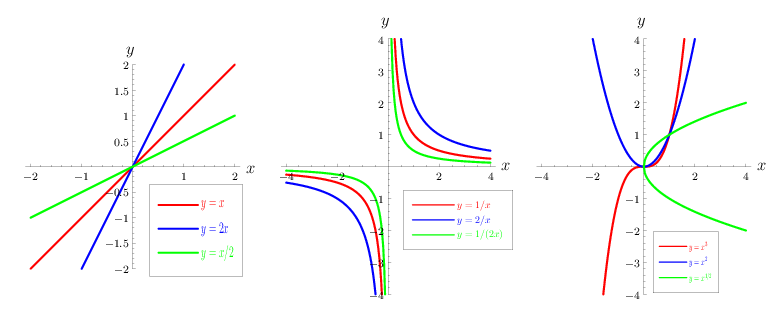
| + | ==Power function== | ||
| + | |||
| + | <center><asy> | ||
| + | import graph; | ||
| + | picture whole; | ||
| + | |||
| + | real sc=0.8; | ||
| + | |||
| + | draw ( graph( new real(real x) {return x;}, -2, 2), red+1.2, "$y=x$" ); | ||
| + | draw ( graph( new real(real x) {return 2x;}, -1, 1), blue+1.2, "$y=2x$" ); | ||
| + | draw ( graph( new real(real x) {return x/2;}, -2, 2), green+1.2, "$y=x/2$" ); | ||
| + | |||
| + | xaxis(-2.1,2.1, LeftTicks(Label(fontsize(8pt)),Step=1,step=0.2,Size=2,size=1,NoZero)); | ||
| + | yaxis(-2,2, RightTicks(Label(fontsize(8pt)),Step=0.5,step=0.1,Size=2,size=1,NoZero)); | ||
| + | labelx("$x$",(2.3,0.25)); | ||
| + | labely("$y$",(0.15,2.3)); | ||
| + | |||
| + | add(scale(0.72sc,1.2sc)*legend(),(0.5,-0.75)); | ||
| + | |||
| + | real mrg=1.3; | ||
| + | draw( scale(mrg)*box((-2,-2),(2,2)), white ); | ||
| + | |||
| + | add (whole,shift(-sc*230,0)*currentpicture.fit(sc*mrg*6.5cm)); | ||
| + | erase(); | ||
| + | |||
| + | |||
| + | draw ( graph( new real(real x) {return 1/x;}, -4, -0.25), red+1.2, "$y=1/x$" ); | ||
| + | draw ( graph( new real(real x) {return 1/x;}, 0.25, 4), red+1.2 ); | ||
| + | draw ( graph( new real(real x) {return 2/x;}, -4, -0.5), blue+1.2, "$y=2/x$" ); | ||
| + | draw ( graph( new real(real x) {return 2/x;}, 0.5, 4), blue+1.2 ); | ||
| + | draw ( graph( new real(real x) {return 1/(2x);}, -4, -0.125), green+1.2, "$y=1/(2x)$" ); | ||
| + | draw ( graph( new real(real x) {return 1/(2x);}, 0.125, 4), green+1.2 ); | ||
| + | |||
| + | xaxis(-4.2,4.2, LeftTicks(Label(fontsize(8pt)),Step=2,step=0.5,Size=2,size=1,NoZero)); | ||
| + | yaxis(-4,4, RightTicks(Label(fontsize(8pt)),Step=1,step=0.2,Size=2,size=1,NoZero)); | ||
| + | labelx("$x$",(4.6,0.5)); | ||
| + | labely("$y$",(0.3,4.6)); | ||
| + | |||
| + | add(scale(0.75sc,0.75sc)*legend(),(0.95,-1.2)); | ||
| + | |||
| + | real mrg=1.3; | ||
| + | draw( scale(mrg)*box((-4,-4),(4,4)), white ); | ||
| + | |||
| + | add (whole,shift(0,0)*currentpicture.fit(sc*mrg*6.5cm,mrg*6.5cm,false)); | ||
| + | erase(); | ||
| + | |||
| + | |||
| + | draw ( graph( new real(real x) {return x^3;}, -4^(1/3), 4^(1/3)), red+1.2, "$y=x^3$" ); | ||
| + | draw ( graph( new real(real x) {return x^2;}, -2, 2), blue+1.2, "$y=x^2$" ); | ||
| + | draw ( graph( new real(real x) {return sqrt(x);}, 0, 4), green+1.2, "$y=x^{1/2}$" ); | ||
| + | draw ( graph( new real(real x) {return -sqrt(x);}, 0, 4), green+1.2 ); | ||
| + | |||
| + | xaxis(-4.2,4.2, LeftTicks(Label(fontsize(8pt)),Step=2,step=0.5,Size=2,size=1,NoZero)); | ||
| + | yaxis(-4,4, RightTicks(Label(fontsize(8pt)),Step=1,step=0.2,Size=2,size=1,NoZero)); | ||
| + | labelx("$x$",(4.6,0.5)); | ||
| + | labely("$y$",(0.3,4.6)); | ||
| + | |||
| + | add(scale(0.5sc,0.75sc)*legend(),(0.6,-2.5)); | ||
| + | |||
| + | real mrg=1.3; | ||
| + | draw( scale(mrg)*box((-4,-4),(4,4)), white ); | ||
| + | |||
| + | add (whole,shift(sc*230,0)*currentpicture.fit(sc*mrg*6.5cm,mrg*6.5cm,false)); | ||
| + | erase(); | ||
| + | |||
| + | shipout(whole); | ||
| + | </asy></center> | ||
| + | |||
| + | ==Kolmogorov test== | ||
| + | |||
| + | <center><asy> | ||
| + | |||
| + | srand(2014011); | ||
| + | |||
| + | import stats; | ||
| + | |||
| + | int size = 13; | ||
| + | real [] sample = new real[size+1]; | ||
| + | real lambda = 1.3/size; | ||
| + | real width = 2.0; | ||
| + | |||
| + | for (int k=0; k<size; ++k) { | ||
| + | sample[k] = Gaussrand(); | ||
| + | } | ||
| + | sample[size] = 10; | ||
| + | |||
| + | sample = sort(sample); | ||
| + | |||
| + | // for (real x : sample ) { | ||
| + | // write(x); | ||
| + | // } | ||
| + | |||
| + | real x0 = -10; | ||
| + | int k = 0; | ||
| + | for (real x : sample ) { | ||
| + | filldraw( box( (x0,k/size-lambda), (x,k/size+lambda) ), rgb(0.8,0.8,0.8) ); | ||
| + | draw( (x0,k/size-lambda)..(x,k/size-lambda), currentpen+1.5 ); | ||
| + | draw( (x0,k/size)..(x,k/size), currentpen+1.5 ); | ||
| + | draw( (x0,k/size+lambda)..(x,k/size+lambda), currentpen+1.5 ); | ||
| + | k += 1; | ||
| + | x0 = x; | ||
| + | draw( (x,(k-1)/size-lambda)..(x,k/size+lambda) ); | ||
| + | } | ||
| + | |||
| + | clip( box((-width,-0.005),(width,1.005)) ); | ||
| + | |||
| + | draw ((-width,0)--(width,0),Arrow); | ||
| + | draw ((0,-0.1)--(0,1.3),Arrow); | ||
| + | draw ((-width,1)--(width,1)); | ||
| + | |||
| + | draw ((sample[2],0)..(sample[2],2/size)); | ||
| + | draw ((sample[size-1],0)..(sample[size-1],0.48), dashed); | ||
| + | draw ((sample[size-1],0.7)..(sample[size-1],1-1/size), dashed); | ||
| + | |||
| + | label("$x$",(width,0),S); | ||
| + | label("$y$",(0,1.3),W); | ||
| + | label("$0$",(0,0),SW); | ||
| + | label("$1$",(0,1),NE); | ||
| + | |||
| + | label("$X_{(1)}$",(sample[0],0),S); | ||
| + | label("$X_{(2)}$",(sample[1],0),S); | ||
| + | label("$X_{(3)}$",(sample[2],0),S); | ||
| + | label("$X_{(n)}$",(sample[size-1],0),S); | ||
| + | |||
| + | label("$F_n(x)+\lambda_n(\alpha)$",(-1.55,0.35)); | ||
| + | draw ((-1.35,0.25)..(-1.2,1/size+lambda)); | ||
| + | dot((-1.2,1/size+lambda)); | ||
| + | |||
| + | label("$F_n(x)$",(0.4,0.3)); | ||
| + | draw ((0.4,0.4)..(0.3,8/size)); | ||
| + | dot((0.3,8/size)); | ||
| + | |||
| + | label("$F_n(x)-\lambda_n(\alpha)$",(1.5,0.6)); | ||
| + | draw ((1.6,0.7)..(1.7,1-lambda)); | ||
| + | dot((1.7,1-lambda)); | ||
| + | |||
| + | shipout(scale(100,100)*currentpicture); | ||
| + | </asy></center> | ||
| + | |||
| + | ==Golden ratio== | ||
| + | |||
| + | Strangely, the figure in EoM is erroneous! ED=EB, not BD=EB. | ||
| + | |||
| + | <center><asy> | ||
| + | |||
| + | pair A=(-1,0); | ||
| + | pair B=(0,0); | ||
| + | pair E=(0,0.5); | ||
| + | pair C=A+(0.5*(sqrt(5)-1),0); | ||
| + | pair D=(-1/sqrt(5), 0.5*(1-1/sqrt(5))); | ||
| + | |||
| + | draw( A--B--E--cycle,currentpen+1.5 ); | ||
| + | dot(A,currentpen+3.5); dot(B,currentpen+3.5); dot(E,currentpen+3.5); dot(C,currentpen+3.5); dot(D,currentpen+3.5); | ||
| + | |||
| + | draw( shift(E)*scale(0.5)*unitcircle,currentpen+1 ); | ||
| + | draw( shift(A)*scale(0.5*(sqrt(5)-1))*unitcircle,currentpen+1 ); | ||
| + | |||
| + | draw( shift(B)*scale(0.5)*unitcircle, dashed+red ); | ||
| + | |||
| + | clip(A+(-0.15,-0.15)--B+(0.15,-0.15)--E+(0.15,0.15)--A+(-0.15,0.15)--cycle); | ||
| + | |||
| + | label("$A$",A,S); label("$B$",B,S); label("$C$",C,S); | ||
| + | label("$E$",E,N); label("$D$",D,N); | ||
| + | |||
| + | label( "\small Golden Ratio construction", (-0.5,0.8) ); | ||
| + | |||
| + | shipout(scale(100)*currentpicture); | ||
| + | </asy></center> | ||
| + | |||
| + | |||
| + | |||
| + | |||
| + | |||
| + | |||
| + | |||
| + | |||
| + | [Calculus: ] the art of numbering and measuring exactly a thing whose existence cannot be conceived. (Voltaire, [http://www.fordham.edu/halsall/mod/1778voltaire-newton.asp Letter XVII: On Infinites In Geometry, And Sir Isaac Newton's Chronology]) | ||
| + | |||
| + | And what are these fluxions? The velocities of evanescent increments? They are neither finite quantities, nor quantities infinitely small, nor yet nothing. May we not call them ghosts of departed quantities? (Berkeley, [http://www-history.mcs.st-and.ac.uk/Quotations/Berkeley.html The Analyst]) | ||
| + | |||
| + | |||
| + | WARNING: Asirra, the cat and dog CAPTCHA, is closing permanently on October 6, 2014. Please contact this site's administrator and ask them to switch to a different CAPTCHA. Thank you! | ||
Latest revision as of 20:14, 12 December 2014
Experiments
Note a fine distinction from Ada:

I guess, the reason is that there Asy generates pdf file (converted into png afterwards), and here something else (probably ps).
No, it seems, it generates eps, both here and there. Then, what could be the reason?
More.


Mysterious.
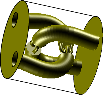
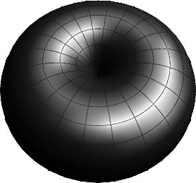
Three dimensions
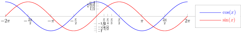
Sinusoid
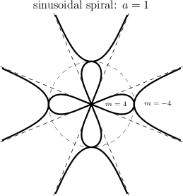
Sinusoidal spiral
Power function
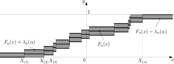
Kolmogorov test
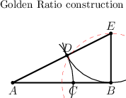
Golden ratio
Strangely, the figure in EoM is erroneous! ED=EB, not BD=EB.
[Calculus: ] the art of numbering and measuring exactly a thing whose existence cannot be conceived. (Voltaire, Letter XVII: On Infinites In Geometry, And Sir Isaac Newton's Chronology)
And what are these fluxions? The velocities of evanescent increments? They are neither finite quantities, nor quantities infinitely small, nor yet nothing. May we not call them ghosts of departed quantities? (Berkeley, The Analyst)
WARNING: Asirra, the cat and dog CAPTCHA, is closing permanently on October 6, 2014. Please contact this site's administrator and ask them to switch to a different CAPTCHA. Thank you!
Boris Tsirelson/sandbox2. Encyclopedia of Mathematics. URL: http://encyclopediaofmath.org/index.php?title=Boris_Tsirelson/sandbox2&oldid=21296