Difference between revisions of "Sturm-Liouville problem"
Ulf Rehmann (talk | contribs) m (tex encoded by computer) |
Ulf Rehmann (talk | contribs) m (Undo revision 48885 by Ulf Rehmann (talk)) Tag: Undo |
||
| Line 1: | Line 1: | ||
| − | < | + | A problem generated by the following equation, where <img align="absmiddle" border="0" src="https://www.encyclopediaofmath.org/legacyimages/s/s090/s090770/s0907701.png" /> varies in a given finite or infinite interval <img align="absmiddle" border="0" src="https://www.encyclopediaofmath.org/legacyimages/s/s090/s090770/s0907702.png" />, |
| − | s0907701.png | ||
| − | |||
| − | |||
| − | |||
| − | |||
| − | |||
| − | |||
| − | + | <table class="eq" style="width:100%;"> <tr><td valign="top" style="width:94%;text-align:center;"><img align="absmiddle" border="0" src="https://www.encyclopediaofmath.org/legacyimages/s/s090/s090770/s0907703.png" /></td> <td valign="top" style="width:5%;text-align:right;">(1)</td></tr></table> | |
| − | |||
| − | + | together with some boundary conditions, where <img align="absmiddle" border="0" src="https://www.encyclopediaofmath.org/legacyimages/s/s090/s090770/s0907704.png" /> and <img align="absmiddle" border="0" src="https://www.encyclopediaofmath.org/legacyimages/s/s090/s090770/s0907705.png" /> are positive, <img align="absmiddle" border="0" src="https://www.encyclopediaofmath.org/legacyimages/s/s090/s090770/s0907706.png" /> is real and <img align="absmiddle" border="0" src="https://www.encyclopediaofmath.org/legacyimages/s/s090/s090770/s0907707.png" /> is a complex parameter. Serious studies of this problem were started by J.Ch. Sturm and J. Liouville. The methods and notions that originated during studies of the Sturm–Liouville problem played an important role in the development of many directions in mathematics and physics. It was and remains a constant source of new ideas and problems in the [[Spectral theory|spectral theory]] of operators and in related problems in analysis. Recently it gained even greater significance, when its relation to certain non-linear evolution equations of mathematical physics were discovered. | |
| − | |||
| − | + | If <img align="absmiddle" border="0" src="https://www.encyclopediaofmath.org/legacyimages/s/s090/s090770/s0907708.png" /> is differentiable and <img align="absmiddle" border="0" src="https://www.encyclopediaofmath.org/legacyimages/s/s090/s090770/s0907709.png" /> is twice differentiable, then, by a substitution, equation (1) can be reduced to (see [[#References|[1]]]) | |
| − | |||
| − | |||
| − | |||
| − | |||
| − | |||
| − | |||
| − | + | <table class="eq" style="width:100%;"> <tr><td valign="top" style="width:94%;text-align:center;"><img align="absmiddle" border="0" src="https://www.encyclopediaofmath.org/legacyimages/s/s090/s090770/s09077010.png" /></td> <td valign="top" style="width:5%;text-align:right;">(2)</td></tr></table> | |
| − | |||
| − | |||
| − | |||
| − | |||
| − | + | It is customary to distinguish between regular and singular problems. A Sturm–Liouville problem for equation (2) is called regular if the interval <img align="absmiddle" border="0" src="https://www.encyclopediaofmath.org/legacyimages/s/s090/s090770/s09077011.png" /> in which <img align="absmiddle" border="0" src="https://www.encyclopediaofmath.org/legacyimages/s/s090/s090770/s09077012.png" /> varies is finite and if the function <img align="absmiddle" border="0" src="https://www.encyclopediaofmath.org/legacyimages/s/s090/s090770/s09077013.png" /> is summable on the entire interval <img align="absmiddle" border="0" src="https://www.encyclopediaofmath.org/legacyimages/s/s090/s090770/s09077014.png" />. If the interval <img align="absmiddle" border="0" src="https://www.encyclopediaofmath.org/legacyimages/s/s090/s090770/s09077015.png" /> is infinite or if <img align="absmiddle" border="0" src="https://www.encyclopediaofmath.org/legacyimages/s/s090/s090770/s09077016.png" /> is not summable (or both), then the problem is called singular. | |
| − | is | ||
| − | |||
| − | + | Below the following possibilities will be considered in some detail: 1) the interval <img align="absmiddle" border="0" src="https://www.encyclopediaofmath.org/legacyimages/s/s090/s090770/s09077017.png" /> is finite (in this case, without loss of generality, one may assume <img align="absmiddle" border="0" src="https://www.encyclopediaofmath.org/legacyimages/s/s090/s090770/s09077018.png" /> and <img align="absmiddle" border="0" src="https://www.encyclopediaofmath.org/legacyimages/s/s090/s090770/s09077019.png" />); 2) <img align="absmiddle" border="0" src="https://www.encyclopediaofmath.org/legacyimages/s/s090/s090770/s09077020.png" />, <img align="absmiddle" border="0" src="https://www.encyclopediaofmath.org/legacyimages/s/s090/s090770/s09077021.png" />; or 3) <img align="absmiddle" border="0" src="https://www.encyclopediaofmath.org/legacyimages/s/s090/s090770/s09077022.png" />, <img align="absmiddle" border="0" src="https://www.encyclopediaofmath.org/legacyimages/s/s090/s090770/s09077023.png" />. | |
| − | |||
| − | |||
| − | + | <img align="absmiddle" border="0" src="https://www.encyclopediaofmath.org/legacyimages/s/s090/s090770/s09077024.png" />. Consider the problem given on the interval <img align="absmiddle" border="0" src="https://www.encyclopediaofmath.org/legacyimages/s/s090/s090770/s09077025.png" /> by equation (2) and the separated boundary conditions | |
| − | |||
| − | |||
| − | |||
| − | |||
| − | |||
| − | |||
| − | + | <table class="eq" style="width:100%;"> <tr><td valign="top" style="width:94%;text-align:center;"><img align="absmiddle" border="0" src="https://www.encyclopediaofmath.org/legacyimages/s/s090/s090770/s09077026.png" /></td> <td valign="top" style="width:5%;text-align:right;">(3)</td></tr></table> | |
| − | |||
| − | |||
| − | |||
| − | |||
| − | |||
| − | |||
| − | + | where <img align="absmiddle" border="0" src="https://www.encyclopediaofmath.org/legacyimages/s/s090/s090770/s09077027.png" /> is a real summable function on <img align="absmiddle" border="0" src="https://www.encyclopediaofmath.org/legacyimages/s/s090/s090770/s09077028.png" />, <img align="absmiddle" border="0" src="https://www.encyclopediaofmath.org/legacyimages/s/s090/s090770/s09077029.png" /> and <img align="absmiddle" border="0" src="https://www.encyclopediaofmath.org/legacyimages/s/s090/s090770/s09077030.png" /> are arbitrary finite or infinite fixed real numbers and <img align="absmiddle" border="0" src="https://www.encyclopediaofmath.org/legacyimages/s/s090/s090770/s09077031.png" /> is a complex parameter. If <img align="absmiddle" border="0" src="https://www.encyclopediaofmath.org/legacyimages/s/s090/s090770/s09077032.png" /> <img align="absmiddle" border="0" src="https://www.encyclopediaofmath.org/legacyimages/s/s090/s090770/s09077033.png" />, then the first (second) condition in (3) is replaced by <img align="absmiddle" border="0" src="https://www.encyclopediaofmath.org/legacyimages/s/s090/s090770/s09077034.png" /> <img align="absmiddle" border="0" src="https://www.encyclopediaofmath.org/legacyimages/s/s090/s090770/s09077035.png" />. To be specific it is further assumed that all numbers occurring in the boundary conditions are finite. | |
| − | |||
| − | |||
| − | + | The number <img align="absmiddle" border="0" src="https://www.encyclopediaofmath.org/legacyimages/s/s090/s090770/s09077036.png" /> is called an eigenvalue for the problem (2), (3) if for <img align="absmiddle" border="0" src="https://www.encyclopediaofmath.org/legacyimages/s/s090/s090770/s09077037.png" /> equation (2) has a non-trivial solution <img align="absmiddle" border="0" src="https://www.encyclopediaofmath.org/legacyimages/s/s090/s090770/s09077038.png" /> that satisfies (3); the function <img align="absmiddle" border="0" src="https://www.encyclopediaofmath.org/legacyimages/s/s090/s090770/s09077039.png" /> is then called the eigenfunction corresponding to the eigenvalue <img align="absmiddle" border="0" src="https://www.encyclopediaofmath.org/legacyimages/s/s090/s090770/s09077040.png" />. | |
| − | |||
| − | |||
| − | |||
| − | + | The eigenvalues for the boundary value problem (2), (3) are real; to the distinct eigenvalues correspond linearly independent eigenfunctions (since <img align="absmiddle" border="0" src="https://www.encyclopediaofmath.org/legacyimages/s/s090/s090770/s09077041.png" /> and the numbers <img align="absmiddle" border="0" src="https://www.encyclopediaofmath.org/legacyimages/s/s090/s090770/s09077042.png" /> are real, the eigenfunctions for the problem (2), (3) can be chosen to be real); eigenfunctions <img align="absmiddle" border="0" src="https://www.encyclopediaofmath.org/legacyimages/s/s090/s090770/s09077043.png" /> and <img align="absmiddle" border="0" src="https://www.encyclopediaofmath.org/legacyimages/s/s090/s090770/s09077044.png" /> corresponding to different eigenvalues are unique and orthogonal, i.e. <img align="absmiddle" border="0" src="https://www.encyclopediaofmath.org/legacyimages/s/s090/s090770/s09077045.png" />. | |
| − | |||
| − | |||
| − | and | ||
| − | |||
| − | |||
| − | |||
| − | |||
| − | |||
| − | |||
| − | + | There exists an unboundedly-increasing sequence of eigenvalues <img align="absmiddle" border="0" src="https://www.encyclopediaofmath.org/legacyimages/s/s090/s090770/s09077046.png" /> for the boundary value problem (2), (3); moreover, the eigenfunction <img align="absmiddle" border="0" src="https://www.encyclopediaofmath.org/legacyimages/s/s090/s090770/s09077047.png" /> corresponding to the eigenvalue <img align="absmiddle" border="0" src="https://www.encyclopediaofmath.org/legacyimages/s/s090/s090770/s09077048.png" /> has precisely <img align="absmiddle" border="0" src="https://www.encyclopediaofmath.org/legacyimages/s/s090/s090770/s09077049.png" /> zeros in the interval <img align="absmiddle" border="0" src="https://www.encyclopediaofmath.org/legacyimages/s/s090/s090770/s09077050.png" />. | |
| − | |||
| − | |||
| − | |||
| − | |||
| − | + | Let <img align="absmiddle" border="0" src="https://www.encyclopediaofmath.org/legacyimages/s/s090/s090770/s09077051.png" /> be the Sobolev space of complex-valued functions on the interval <img align="absmiddle" border="0" src="https://www.encyclopediaofmath.org/legacyimages/s/s090/s090770/s09077052.png" /> that have <img align="absmiddle" border="0" src="https://www.encyclopediaofmath.org/legacyimages/s/s090/s090770/s09077053.png" /> absolutely-continuous derivatives and with <img align="absmiddle" border="0" src="https://www.encyclopediaofmath.org/legacyimages/s/s090/s090770/s09077054.png" />-th derivatives summable on <img align="absmiddle" border="0" src="https://www.encyclopediaofmath.org/legacyimages/s/s090/s090770/s09077055.png" />. If <img align="absmiddle" border="0" src="https://www.encyclopediaofmath.org/legacyimages/s/s090/s090770/s09077056.png" />, then the eigenvalues <img align="absmiddle" border="0" src="https://www.encyclopediaofmath.org/legacyimages/s/s090/s090770/s09077057.png" /> of the boundary value problem (2), (3) for large <img align="absmiddle" border="0" src="https://www.encyclopediaofmath.org/legacyimages/s/s090/s090770/s09077058.png" /> satisfy the following asymptotic equation (see [[#References|[4]]]): | |
| − | and | ||
| − | |||
| − | |||
| − | |||
| − | + | <table class="eq" style="width:100%;"> <tr><td valign="top" style="width:94%;text-align:center;"><img align="absmiddle" border="0" src="https://www.encyclopediaofmath.org/legacyimages/s/s090/s090770/s09077059.png" /></td> </tr></table> | |
| − | |||
| − | |||
| − | |||
| − | |||
| − | + | <table class="eq" style="width:100%;"> <tr><td valign="top" style="width:94%;text-align:center;"><img align="absmiddle" border="0" src="https://www.encyclopediaofmath.org/legacyimages/s/s090/s090770/s09077060.png" /></td> </tr></table> | |
| − | |||
| − | |||
| − | |||
| − | |||
| − | |||
| − | |||
| − | |||
| − | |||
| − | + | where <img align="absmiddle" border="0" src="https://www.encyclopediaofmath.org/legacyimages/s/s090/s090770/s09077061.png" /> are numbers independent of <img align="absmiddle" border="0" src="https://www.encyclopediaofmath.org/legacyimages/s/s090/s090770/s09077062.png" />, | |
| − | |||
| − | |||
| − | |||
| − | |||
| − | + | <table class="eq" style="width:100%;"> <tr><td valign="top" style="width:94%;text-align:center;"><img align="absmiddle" border="0" src="https://www.encyclopediaofmath.org/legacyimages/s/s090/s090770/s09077063.png" /></td> </tr></table> | |
| − | |||
| − | + | <table class="eq" style="width:100%;"> <tr><td valign="top" style="width:94%;text-align:center;"><img align="absmiddle" border="0" src="https://www.encyclopediaofmath.org/legacyimages/s/s090/s090770/s09077064.png" /></td> </tr></table> | |
| − | |||
| − | |||
| − | |||
| − | |||
| − | |||
| − | |||
| − | |||
| − | |||
| − | |||
| − | |||
| − | + | <table class="eq" style="width:100%;"> <tr><td valign="top" style="width:94%;text-align:center;"><img align="absmiddle" border="0" src="https://www.encyclopediaofmath.org/legacyimages/s/s090/s090770/s09077065.png" /></td> </tr></table> | |
| − | |||
| − | + | <img align="absmiddle" border="0" src="https://www.encyclopediaofmath.org/legacyimages/s/s090/s090770/s09077066.png" /> does not depend on <img align="absmiddle" border="0" src="https://www.encyclopediaofmath.org/legacyimages/s/s090/s090770/s09077067.png" />, and | |
| − | |||
| − | |||
| − | |||
| − | |||
| − | |||
| − | |||
| − | + | <table class="eq" style="width:100%;"> <tr><td valign="top" style="width:94%;text-align:center;"><img align="absmiddle" border="0" src="https://www.encyclopediaofmath.org/legacyimages/s/s090/s090770/s09077068.png" /></td> </tr></table> | |
| − | |||
| − | |||
| − | |||
| − | |||
| − | |||
| − | |||
| − | + | The above implies, in particular, that if <img align="absmiddle" border="0" src="https://www.encyclopediaofmath.org/legacyimages/s/s090/s090770/s09077069.png" />, then | |
| − | |||
| − | |||
| − | |||
| − | |||
| − | |||
| − | |||
| − | |||
| − | + | <table class="eq" style="width:100%;"> <tr><td valign="top" style="width:94%;text-align:center;"><img align="absmiddle" border="0" src="https://www.encyclopediaofmath.org/legacyimages/s/s090/s090770/s09077070.png" /></td> </tr></table> | |
| − | |||
| − | |||
| − | |||
| − | |||
| − | |||
| − | |||
| − | |||
| − | |||
| − | |||
| − | |||
| − | |||
| − | |||
| − | |||
| − | |||
| − | |||
| − | |||
where | where | ||
| − | + | <table class="eq" style="width:100%;"> <tr><td valign="top" style="width:94%;text-align:center;"><img align="absmiddle" border="0" src="https://www.encyclopediaofmath.org/legacyimages/s/s090/s090770/s09077071.png" /></td> </tr></table> | |
| − | |||
| − | |||
| − | |||
| − | |||
| − | |||
| − | |||
| − | |||
| − | |||
| − | Thus, the series | + | Thus, the series <img align="absmiddle" border="0" src="https://www.encyclopediaofmath.org/legacyimages/s/s090/s090770/s09077072.png" /> is convergent. Its sum is called the regularized trace of the problem (2), (3) (see [[#References|[13]]]): |
| − | is convergent. Its sum is called the regularized trace of the problem (2), (3) (see [[#References|[13]]]): | ||
| − | + | <table class="eq" style="width:100%;"> <tr><td valign="top" style="width:94%;text-align:center;"><img align="absmiddle" border="0" src="https://www.encyclopediaofmath.org/legacyimages/s/s090/s090770/s09077073.png" /></td> </tr></table> | |
| − | |||
| − | + | Let <img align="absmiddle" border="0" src="https://www.encyclopediaofmath.org/legacyimages/s/s090/s090770/s09077074.png" /> be the orthonormal eigenfunctions of the problem (2), (3) corresponding to the eigenvalues <img align="absmiddle" border="0" src="https://www.encyclopediaofmath.org/legacyimages/s/s090/s090770/s09077075.png" />. For any function <img align="absmiddle" border="0" src="https://www.encyclopediaofmath.org/legacyimages/s/s090/s090770/s09077076.png" /> the so-called Parseval equality holds: | |
| − | |||
| − | |||
| − | |||
| − | |||
| − | |||
| − | |||
| − | + | <table class="eq" style="width:100%;"> <tr><td valign="top" style="width:94%;text-align:center;"><img align="absmiddle" border="0" src="https://www.encyclopediaofmath.org/legacyimages/s/s090/s090770/s09077077.png" /></td> </tr></table> | |
| − | |||
| − | |||
| − | |||
| − | |||
| − | |||
| − | |||
| − | |||
where | where | ||
| − | + | <table class="eq" style="width:100%;"> <tr><td valign="top" style="width:94%;text-align:center;"><img align="absmiddle" border="0" src="https://www.encyclopediaofmath.org/legacyimages/s/s090/s090770/s09077078.png" /></td> </tr></table> | |
| − | |||
| − | |||
and the following formula for eigenfunction expansion is valid: | and the following formula for eigenfunction expansion is valid: | ||
| − | + | <table class="eq" style="width:100%;"> <tr><td valign="top" style="width:94%;text-align:center;"><img align="absmiddle" border="0" src="https://www.encyclopediaofmath.org/legacyimages/s/s090/s090770/s09077079.png" /></td> <td valign="top" style="width:5%;text-align:right;">(4)</td></tr></table> | |
| − | |||
| − | |||
| − | where the series converges in the metric of | + | where the series converges in the metric of <img align="absmiddle" border="0" src="https://www.encyclopediaofmath.org/legacyimages/s/s090/s090770/s09077080.png" />. Completeness and expansion theorems for a regular Sturm–Liouville problem were first proved by V.A. Steklov [[#References|[14]]]. |
| − | Completeness and expansion theorems for a regular Sturm–Liouville problem were first proved by V.A. Steklov [[#References|[14]]]. | ||
| − | If the function | + | If the function <img align="absmiddle" border="0" src="https://www.encyclopediaofmath.org/legacyimages/s/s090/s090770/s09077081.png" /> has a continuous second derivative and satisfies the boundary conditions (3), then the following assertions hold (see [[#References|[15]]]): |
| − | has a continuous second derivative and satisfies the boundary conditions (3), then the following assertions hold (see [[#References|[15]]]): | ||
| − | a) the series (4) converges absolutely and uniformly on | + | a) the series (4) converges absolutely and uniformly on <img align="absmiddle" border="0" src="https://www.encyclopediaofmath.org/legacyimages/s/s090/s090770/s09077082.png" /> to <img align="absmiddle" border="0" src="https://www.encyclopediaofmath.org/legacyimages/s/s090/s090770/s09077083.png" />; |
| − | to | ||
| − | b) the once-differentiated series (4) converges absolutely and uniformly on | + | b) the once-differentiated series (4) converges absolutely and uniformly on <img align="absmiddle" border="0" src="https://www.encyclopediaofmath.org/legacyimages/s/s090/s090770/s09077084.png" /> to <img align="absmiddle" border="0" src="https://www.encyclopediaofmath.org/legacyimages/s/s090/s090770/s09077085.png" />; |
| − | to | ||
| − | c) at any point where | + | c) at any point where <img align="absmiddle" border="0" src="https://www.encyclopediaofmath.org/legacyimages/s/s090/s090770/s09077086.png" /> satisfies some local condition of expansion in a Fourier series (e.g. is of bounded variation), the twice-differentiated series (4) converges to <img align="absmiddle" border="0" src="https://www.encyclopediaofmath.org/legacyimages/s/s090/s090770/s09077087.png" />. |
| − | satisfies some local condition of expansion in a Fourier series (e.g. is of bounded variation), the twice-differentiated series (4) converges to | ||
| − | For any function | + | For any function <img align="absmiddle" border="0" src="https://www.encyclopediaofmath.org/legacyimages/s/s090/s090770/s09077088.png" /> the series (4) is uniformly equiconvergent with the Fourier cosine series of <img align="absmiddle" border="0" src="https://www.encyclopediaofmath.org/legacyimages/s/s090/s090770/s09077089.png" />, i.e. |
| − | the series (4) is uniformly equiconvergent with the Fourier cosine series of | ||
| − | i.e. | ||
| − | + | <table class="eq" style="width:100%;"> <tr><td valign="top" style="width:94%;text-align:center;"><img align="absmiddle" border="0" src="https://www.encyclopediaofmath.org/legacyimages/s/s090/s090770/s09077090.png" /></td> </tr></table> | |
| − | |||
| − | - | ||
| − | |||
where | where | ||
| − | + | <table class="eq" style="width:100%;"> <tr><td valign="top" style="width:94%;text-align:center;"><img align="absmiddle" border="0" src="https://www.encyclopediaofmath.org/legacyimages/s/s090/s090770/s09077091.png" /></td> </tr></table> | |
| − | |||
| − | |||
| − | + | <table class="eq" style="width:100%;"> <tr><td valign="top" style="width:94%;text-align:center;"><img align="absmiddle" border="0" src="https://www.encyclopediaofmath.org/legacyimages/s/s090/s090770/s09077092.png" /></td> </tr></table> | |
| − | |||
| − | |||
| − | |||
| − | + | This means that the expansion of <img align="absmiddle" border="0" src="https://www.encyclopediaofmath.org/legacyimages/s/s090/s090770/s09077093.png" /> with respect to the eigenfunctions of the boundary value problem (2), (3) converges under the same conditions as the expansion of <img align="absmiddle" border="0" src="https://www.encyclopediaofmath.org/legacyimages/s/s090/s090770/s09077094.png" /> in a Fourier cosine series (see [[#References|[1]]], [[#References|[4]]]). | |
| − | |||
| − | |||
| − | + | <img align="absmiddle" border="0" src="https://www.encyclopediaofmath.org/legacyimages/s/s090/s090770/s09077095.png" />. The differential equation (2) is considered on the half-line <img align="absmiddle" border="0" src="https://www.encyclopediaofmath.org/legacyimages/s/s090/s090770/s09077096.png" /> with a boundary condition at zero: | |
| − | |||
| − | |||
| − | + | <table class="eq" style="width:100%;"> <tr><td valign="top" style="width:94%;text-align:center;"><img align="absmiddle" border="0" src="https://www.encyclopediaofmath.org/legacyimages/s/s090/s090770/s09077097.png" /></td> <td valign="top" style="width:5%;text-align:right;">(5)</td></tr></table> | |
| − | |||
| − | |||
| − | + | The function <img align="absmiddle" border="0" src="https://www.encyclopediaofmath.org/legacyimages/s/s090/s090770/s09077098.png" /> is assumed to be real and summable on any finite subinterval of <img align="absmiddle" border="0" src="https://www.encyclopediaofmath.org/legacyimages/s/s090/s090770/s09077099.png" /> and <img align="absmiddle" border="0" src="https://www.encyclopediaofmath.org/legacyimages/s/s090/s090770/s090770100.png" /> is assumed to be real. | |
| − | |||
| − | |||
| − | + | Let <img align="absmiddle" border="0" src="https://www.encyclopediaofmath.org/legacyimages/s/s090/s090770/s090770101.png" /> be a solution of (2) with the initial conditions <img align="absmiddle" border="0" src="https://www.encyclopediaofmath.org/legacyimages/s/s090/s090770/s090770102.png" />, <img align="absmiddle" border="0" src="https://www.encyclopediaofmath.org/legacyimages/s/s090/s090770/s090770103.png" /> (so that <img align="absmiddle" border="0" src="https://www.encyclopediaofmath.org/legacyimages/s/s090/s090770/s090770104.png" /> satisfies also the boundary condition (5)). Let <img align="absmiddle" border="0" src="https://www.encyclopediaofmath.org/legacyimages/s/s090/s090770/s090770105.png" /> be any function from <img align="absmiddle" border="0" src="https://www.encyclopediaofmath.org/legacyimages/s/s090/s090770/s090770106.png" /> and let <img align="absmiddle" border="0" src="https://www.encyclopediaofmath.org/legacyimages/s/s090/s090770/s090770107.png" />, where <img align="absmiddle" border="0" src="https://www.encyclopediaofmath.org/legacyimages/s/s090/s090770/s090770108.png" /> is an arbitrary finite positive number. For any function <img align="absmiddle" border="0" src="https://www.encyclopediaofmath.org/legacyimages/s/s090/s090770/s090770109.png" /> and any number <img align="absmiddle" border="0" src="https://www.encyclopediaofmath.org/legacyimages/s/s090/s090770/s090770110.png" /> there is at least one decreasing function <img align="absmiddle" border="0" src="https://www.encyclopediaofmath.org/legacyimages/s/s090/s090770/s090770111.png" />, <img align="absmiddle" border="0" src="https://www.encyclopediaofmath.org/legacyimages/s/s090/s090770/s090770112.png" />, independent of <img align="absmiddle" border="0" src="https://www.encyclopediaofmath.org/legacyimages/s/s090/s090770/s090770113.png" />, that has the following properties: | |
| − | |||
| − | and | ||
| − | is | ||
| − | + | a) there is a function <img align="absmiddle" border="0" src="https://www.encyclopediaofmath.org/legacyimages/s/s090/s090770/s090770114.png" />, which is the limit of <img align="absmiddle" border="0" src="https://www.encyclopediaofmath.org/legacyimages/s/s090/s090770/s090770115.png" /> for <img align="absmiddle" border="0" src="https://www.encyclopediaofmath.org/legacyimages/s/s090/s090770/s090770116.png" /> in the metric of <img align="absmiddle" border="0" src="https://www.encyclopediaofmath.org/legacyimages/s/s090/s090770/s090770117.png" /> (the space of <img align="absmiddle" border="0" src="https://www.encyclopediaofmath.org/legacyimages/s/s090/s090770/s090770118.png" />-measurable functions <img align="absmiddle" border="0" src="https://www.encyclopediaofmath.org/legacyimages/s/s090/s090770/s090770119.png" /> for which <img align="absmiddle" border="0" src="https://www.encyclopediaofmath.org/legacyimages/s/s090/s090770/s090770120.png" />), i.e. | |
| − | |||
| − | |||
| − | |||
| − | |||
| − | |||
| − | |||
| − | |||
| − | |||
| − | |||
| − | |||
| − | |||
| − | |||
| − | |||
| − | + | <table class="eq" style="width:100%;"> <tr><td valign="top" style="width:94%;text-align:center;"><img align="absmiddle" border="0" src="https://www.encyclopediaofmath.org/legacyimages/s/s090/s090770/s090770121.png" /></td> </tr></table> | |
| − | |||
| − | |||
| − | |||
| − | |||
| − | |||
| − | |||
| − | |||
| − | |||
| − | |||
| − | |||
| − | |||
b) the Parseval equality is valid: | b) the Parseval equality is valid: | ||
| − | + | <table class="eq" style="width:100%;"> <tr><td valign="top" style="width:94%;text-align:center;"><img align="absmiddle" border="0" src="https://www.encyclopediaofmath.org/legacyimages/s/s090/s090770/s090770122.png" /></td> </tr></table> | |
| − | |||
| − | |||
| − | |||
| − | The function | + | The function <img align="absmiddle" border="0" src="https://www.encyclopediaofmath.org/legacyimages/s/s090/s090770/s090770123.png" /> is called the spectral function (or spectral density) for the boundary value problem (2), (5) (see [[#References|[9]]]–[[#References|[11]]]). |
| − | is called the spectral function (or spectral density) for the boundary value problem (2), (5) (see [[#References|[9]]]–[[#References|[11]]]). | ||
| − | For the spectral function | + | For the spectral function <img align="absmiddle" border="0" src="https://www.encyclopediaofmath.org/legacyimages/s/s090/s090770/s090770124.png" /> of the problem (2), (5) the following asymptotic formula is true (see [[#References|[16]]]) (for a more precise form, see ): |
| − | of the problem (2), (5) the following asymptotic formula is true (see [[#References|[16]]]) (for a more precise form, see ): | ||
| − | + | <table class="eq" style="width:100%;"> <tr><td valign="top" style="width:94%;text-align:center;"><img align="absmiddle" border="0" src="https://www.encyclopediaofmath.org/legacyimages/s/s090/s090770/s090770125.png" /></td> </tr></table> | |
| − | |||
| − | |||
| − | |||
| − | |||
| − | + | <table class="eq" style="width:100%;"> <tr><td valign="top" style="width:94%;text-align:center;"><img align="absmiddle" border="0" src="https://www.encyclopediaofmath.org/legacyimages/s/s090/s090770/s090770126.png" /></td> </tr></table> | |
| − | |||
| − | |||
| − | |||
| − | |||
| − | |||
| − | The following equiconvergence theorem is valid : For an arbitrary function | + | The following equiconvergence theorem is valid : For an arbitrary function <img align="absmiddle" border="0" src="https://www.encyclopediaofmath.org/legacyimages/s/s090/s090770/s090770127.png" />, let |
| − | let | ||
| − | + | <table class="eq" style="width:100%;"> <tr><td valign="top" style="width:94%;text-align:center;"><img align="absmiddle" border="0" src="https://www.encyclopediaofmath.org/legacyimages/s/s090/s090770/s090770128.png" /></td> </tr></table> | |
| − | |||
| − | |||
| − | + | <table class="eq" style="width:100%;"> <tr><td valign="top" style="width:94%;text-align:center;"><img align="absmiddle" border="0" src="https://www.encyclopediaofmath.org/legacyimages/s/s090/s090770/s090770129.png" /></td> </tr></table> | |
| − | |||
| − | |||
| − | (the integrals converge in the metrics of | + | (the integrals converge in the metrics of <img align="absmiddle" border="0" src="https://www.encyclopediaofmath.org/legacyimages/s/s090/s090770/s090770130.png" /> and <img align="absmiddle" border="0" src="https://www.encyclopediaofmath.org/legacyimages/s/s090/s090770/s090770131.png" />, respectively); then for any fixed <img align="absmiddle" border="0" src="https://www.encyclopediaofmath.org/legacyimages/s/s090/s090770/s090770132.png" /> the integral |
| − | and | ||
| − | respectively); then for any fixed | ||
| − | the integral | ||
| − | + | <table class="eq" style="width:100%;"> <tr><td valign="top" style="width:94%;text-align:center;"><img align="absmiddle" border="0" src="https://www.encyclopediaofmath.org/legacyimages/s/s090/s090770/s090770133.png" /></td> </tr></table> | |
| − | |||
| − | |||
| − | converges absolutely and uniformly with respect to | + | converges absolutely and uniformly with respect to <img align="absmiddle" border="0" src="https://www.encyclopediaofmath.org/legacyimages/s/s090/s090770/s090770134.png" />, and |
| − | and | ||
| − | + | <table class="eq" style="width:100%;"> <tr><td valign="top" style="width:94%;text-align:center;"><img align="absmiddle" border="0" src="https://www.encyclopediaofmath.org/legacyimages/s/s090/s090770/s090770135.png" /></td> </tr></table> | |
| − | |||
| − | |||
| − | |||
| − | + | <table class="eq" style="width:100%;"> <tr><td valign="top" style="width:94%;text-align:center;"><img align="absmiddle" border="0" src="https://www.encyclopediaofmath.org/legacyimages/s/s090/s090770/s090770136.png" /></td> </tr></table> | |
| − | - | ||
| − | + | Let problem (2), (5) have a discrete spectrum, i.e. let its spectrum consist of a countable number of eigenvalues <img align="absmiddle" border="0" src="https://www.encyclopediaofmath.org/legacyimages/s/s090/s090770/s090770137.png" /> with a unique limit point at infinity. Under certain restrictions on the function <img align="absmiddle" border="0" src="https://www.encyclopediaofmath.org/legacyimages/s/s090/s090770/s090770138.png" />, for the function <img align="absmiddle" border="0" src="https://www.encyclopediaofmath.org/legacyimages/s/s090/s090770/s090770139.png" />, i.e. the number of eigenvalues less than <img align="absmiddle" border="0" src="https://www.encyclopediaofmath.org/legacyimages/s/s090/s090770/s090770140.png" />, the following asymptotic formula is valid: | |
| − | |||
| − | |||
| − | |||
| − | + | <table class="eq" style="width:100%;"> <tr><td valign="top" style="width:94%;text-align:center;"><img align="absmiddle" border="0" src="https://www.encyclopediaofmath.org/legacyimages/s/s090/s090770/s090770141.png" /></td> </tr></table> | |
| − | |||
| − | |||
| − | |||
| − | |||
| − | + | Simultaneously with <img align="absmiddle" border="0" src="https://www.encyclopediaofmath.org/legacyimages/s/s090/s090770/s090770142.png" />, a second solution <img align="absmiddle" border="0" src="https://www.encyclopediaofmath.org/legacyimages/s/s090/s090770/s090770143.png" /> of equation (2) is introduced, satisfying the conditions <img align="absmiddle" border="0" src="https://www.encyclopediaofmath.org/legacyimages/s/s090/s090770/s090770144.png" />, <img align="absmiddle" border="0" src="https://www.encyclopediaofmath.org/legacyimages/s/s090/s090770/s090770145.png" />, so that <img align="absmiddle" border="0" src="https://www.encyclopediaofmath.org/legacyimages/s/s090/s090770/s090770146.png" /> and <img align="absmiddle" border="0" src="https://www.encyclopediaofmath.org/legacyimages/s/s090/s090770/s090770147.png" /> form a [[Fundamental system of solutions|fundamental system of solutions]] of (2). For a fixed <img align="absmiddle" border="0" src="https://www.encyclopediaofmath.org/legacyimages/s/s090/s090770/s090770148.png" /> <img align="absmiddle" border="0" src="https://www.encyclopediaofmath.org/legacyimages/s/s090/s090770/s090770149.png" /> and <img align="absmiddle" border="0" src="https://www.encyclopediaofmath.org/legacyimages/s/s090/s090770/s090770150.png" /> the following fractional-linear function is considered: | |
| − | |||
| − | |||
| − | |||
| − | |||
| − | |||
| − | + | <table class="eq" style="width:100%;"> <tr><td valign="top" style="width:94%;text-align:center;"><img align="absmiddle" border="0" src="https://www.encyclopediaofmath.org/legacyimages/s/s090/s090770/s090770151.png" /></td> </tr></table> | |
| − | |||
| − | |||
| − | |||
| − | |||
| − | |||
| − | |||
| − | |||
| − | |||
| − | |||
| − | + | When the independent variable <img align="absmiddle" border="0" src="https://www.encyclopediaofmath.org/legacyimages/s/s090/s090770/s090770152.png" /> varies on the real line, the point <img align="absmiddle" border="0" src="https://www.encyclopediaofmath.org/legacyimages/s/s090/s090770/s090770153.png" /> describes a circle bounding a disc <img align="absmiddle" border="0" src="https://www.encyclopediaofmath.org/legacyimages/s/s090/s090770/s090770154.png" />. It always lies in the same half-plane (lower or upper) as <img align="absmiddle" border="0" src="https://www.encyclopediaofmath.org/legacyimages/s/s090/s090770/s090770155.png" />. When <img align="absmiddle" border="0" src="https://www.encyclopediaofmath.org/legacyimages/s/s090/s090770/s090770156.png" /> increases, <img align="absmiddle" border="0" src="https://www.encyclopediaofmath.org/legacyimages/s/s090/s090770/s090770157.png" /> shrinks, i.e. for <img align="absmiddle" border="0" src="https://www.encyclopediaofmath.org/legacyimages/s/s090/s090770/s090770158.png" /> the disc <img align="absmiddle" border="0" src="https://www.encyclopediaofmath.org/legacyimages/s/s090/s090770/s090770159.png" /> lies entirely inside the disc <img align="absmiddle" border="0" src="https://www.encyclopediaofmath.org/legacyimages/s/s090/s090770/s090770160.png" />. There is (for <img align="absmiddle" border="0" src="https://www.encyclopediaofmath.org/legacyimages/s/s090/s090770/s090770161.png" />) a limit disc or a point <img align="absmiddle" border="0" src="https://www.encyclopediaofmath.org/legacyimages/s/s090/s090770/s090770162.png" />; if | |
| − | |||
| − | + | <table class="eq" style="width:100%;"> <tr><td valign="top" style="width:94%;text-align:center;"><img align="absmiddle" border="0" src="https://www.encyclopediaofmath.org/legacyimages/s/s090/s090770/s090770163.png" /></td> <td valign="top" style="width:5%;text-align:right;">(6)</td></tr></table> | |
| − | |||
| − | |||
| − | |||
| − | + | then <img align="absmiddle" border="0" src="https://www.encyclopediaofmath.org/legacyimages/s/s090/s090770/s090770164.png" /> is a disc, otherwise it is a point (see [[#References|[10]]]). If condition (6) is fulfilled for some non-real value of <img align="absmiddle" border="0" src="https://www.encyclopediaofmath.org/legacyimages/s/s090/s090770/s090770165.png" />, then it is fulfilled for all values of <img align="absmiddle" border="0" src="https://www.encyclopediaofmath.org/legacyimages/s/s090/s090770/s090770166.png" />. In the case of a limit disc, for any value of <img align="absmiddle" border="0" src="https://www.encyclopediaofmath.org/legacyimages/s/s090/s090770/s090770167.png" /> all solutions of (2) belong to <img align="absmiddle" border="0" src="https://www.encyclopediaofmath.org/legacyimages/s/s090/s090770/s090770168.png" />, and in the case of a limit point, for any non-real value of <img align="absmiddle" border="0" src="https://www.encyclopediaofmath.org/legacyimages/s/s090/s090770/s090770169.png" /> this equation has the solution <img align="absmiddle" border="0" src="https://www.encyclopediaofmath.org/legacyimages/s/s090/s090770/s090770170.png" />, which belongs to <img align="absmiddle" border="0" src="https://www.encyclopediaofmath.org/legacyimages/s/s090/s090770/s090770171.png" />, where <img align="absmiddle" border="0" src="https://www.encyclopediaofmath.org/legacyimages/s/s090/s090770/s090770172.png" /> is the limit point <img align="absmiddle" border="0" src="https://www.encyclopediaofmath.org/legacyimages/s/s090/s090770/s090770173.png" />. | |
| − | |||
| − | |||
| − | |||
| − | |||
| − | |||
| − | |||
| − | |||
| − | |||
| − | |||
| − | |||
| − | |||
| − | + | If <img align="absmiddle" border="0" src="https://www.encyclopediaofmath.org/legacyimages/s/s090/s090770/s090770174.png" />, where <img align="absmiddle" border="0" src="https://www.encyclopediaofmath.org/legacyimages/s/s090/s090770/s090770175.png" /> is some positive constant, then the case of a limit point holds (see [[#References|[19]]]); for more general results see [[#References|[20]]], [[#References|[21]]]. | |
| − | |||
| − | |||
| − | + | <img align="absmiddle" border="0" src="https://www.encyclopediaofmath.org/legacyimages/s/s090/s090770/s090770176.png" />. Consider now equation (2) on the whole line <img align="absmiddle" border="0" src="https://www.encyclopediaofmath.org/legacyimages/s/s090/s090770/s090770177.png" /> under the assumption that <img align="absmiddle" border="0" src="https://www.encyclopediaofmath.org/legacyimages/s/s090/s090770/s090770178.png" /> is a real summable function on every finite subinterval of <img align="absmiddle" border="0" src="https://www.encyclopediaofmath.org/legacyimages/s/s090/s090770/s090770179.png" />. Let <img align="absmiddle" border="0" src="https://www.encyclopediaofmath.org/legacyimages/s/s090/s090770/s090770180.png" />, <img align="absmiddle" border="0" src="https://www.encyclopediaofmath.org/legacyimages/s/s090/s090770/s090770181.png" /> be the solutions of (2) satisfying the conditions <img align="absmiddle" border="0" src="https://www.encyclopediaofmath.org/legacyimages/s/s090/s090770/s090770182.png" />, <img align="absmiddle" border="0" src="https://www.encyclopediaofmath.org/legacyimages/s/s090/s090770/s090770183.png" />. | |
| − | |||
| − | |||
| − | |||
| − | |||
| − | |||
| − | |||
| − | |||
| − | |||
| − | |||
| − | |||
| − | |||
| − | |||
| − | |||
| − | |||
| − | |||
| − | Consider now equation (2) on the whole line | ||
| − | under the assumption that | ||
| − | is a real summable function on every finite subinterval of | ||
| − | Let | ||
| − | |||
| − | be the solutions of (2) satisfying the conditions | ||
| − | |||
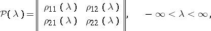
There is at least one real symmetric non-decreasing matrix-function | There is at least one real symmetric non-decreasing matrix-function | ||
| − | + | <table class="eq" style="width:100%;"> <tr><td valign="top" style="width:94%;text-align:center;"><img align="absmiddle" border="0" src="https://www.encyclopediaofmath.org/legacyimages/s/s090/s090770/s090770184.png" /></td> </tr></table> | |
| − | |||
with the following properties: | with the following properties: | ||
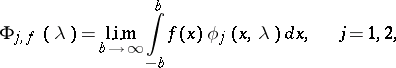
| − | a) for any function | + | a) for any function <img align="absmiddle" border="0" src="https://www.encyclopediaofmath.org/legacyimages/s/s090/s090770/s090770185.png" /> there exist functions <img align="absmiddle" border="0" src="https://www.encyclopediaofmath.org/legacyimages/s/s090/s090770/s090770186.png" />, <img align="absmiddle" border="0" src="https://www.encyclopediaofmath.org/legacyimages/s/s090/s090770/s090770187.png" />, defined by |
| − | there exist functions | ||
| − | |||
| − | defined by | ||
| − | + | <table class="eq" style="width:100%;"> <tr><td valign="top" style="width:94%;text-align:center;"><img align="absmiddle" border="0" src="https://www.encyclopediaofmath.org/legacyimages/s/s090/s090770/s090770188.png" /></td> </tr></table> | |
| − | |||
| − | |||
| − | |||
| − | |||
| − | where the limit is in the metric of | + | where the limit is in the metric of <img align="absmiddle" border="0" src="https://www.encyclopediaofmath.org/legacyimages/s/s090/s090770/s090770189.png" />; |
b) the Parseval equality is valid: | b) the Parseval equality is valid: | ||
| − | + | <table class="eq" style="width:100%;"> <tr><td valign="top" style="width:94%;text-align:center;"><img align="absmiddle" border="0" src="https://www.encyclopediaofmath.org/legacyimages/s/s090/s090770/s090770190.png" /></td> </tr></table> | |
| − | |||
| − | |||
| − | |||
====References==== | ====References==== | ||
<table><TR><TD valign="top">[1]</TD> <TD valign="top"> B.M. Levitan, I.S. Sargsyan, "An introduction to spectral theory" , Amer. Math. Soc. (1975) (Translated from Russian)</TD></TR><TR><TD valign="top">[2]</TD> <TD valign="top"> B.M. Levitan, "Eigenfunction expansions of second-order differential equations" , Moscow-Leningrad (1950) (In Russian)</TD></TR><TR><TD valign="top">[3]</TD> <TD valign="top"> B.M. Levitan, "Generalized translation operators and some of their applications" , Israel Program Sci. Transl. (1964) (Translated from Russian)</TD></TR><TR><TD valign="top">[4]</TD> <TD valign="top"> V.A. Marchenko, "Sturm–Liouville operators and applications" , Birkhäuser (1986) (Translated from Russian)</TD></TR><TR><TD valign="top">[5]</TD> <TD valign="top"> E.C. Titchmarsh, "Eigenfunction expansions associated with second-order differential equations" , '''1''' , Clarendon Press (1962)</TD></TR><TR><TD valign="top">[6]</TD> <TD valign="top"> E.A. Coddington, N. Levinson, "Theory of ordinary differential equations" , McGraw-Hill (1955) pp. Chapts. 13–17</TD></TR><TR><TD valign="top">[7]</TD> <TD valign="top"> M.A. Naimark, "Lineare Differentialoperatoren" , Akademie Verlag (1960) (Translated from Russian)</TD></TR><TR><TD valign="top">[8]</TD> <TD valign="top"> A.G. Kostyuchenko, I.S. Sargsyan, "Distribution of eigenvalues" , Moscow (1979) (In Russian)</TD></TR><TR><TD valign="top">[9]</TD> <TD valign="top"> H. Weyl, "Über gewöhnliche lineare Differentialgleichungen mit singulären Stellen und ihre Eigenfunktionen" ''Gött. Nachr.'' (1909) pp. 37–64</TD></TR><TR><TD valign="top">[10]</TD> <TD valign="top"> H. Weyl, "Über gewöhnliche lineare Differentialgleichungen mit Singularitäten und die Zugehörigen Entwicklungen willküriger Funktionen" ''Math. Ann.'' , '''68''' (1910) pp. 220–269</TD></TR><TR><TD valign="top">[11]</TD> <TD valign="top"> H. Weyl, "Über gewöhnliche lineare Differentialgleichungen mit singulären Stellen und ihre Eigenfunktionen (2)" ''Gött. Nachr.'' (1910) pp. 442–467</TD></TR><TR><TD valign="top">[12]</TD> <TD valign="top"> M.G. Krein, "On the indeterminate case of the Sturm–Liouville boundary problem in the interval <img align="absmiddle" border="0" src="https://www.encyclopediaofmath.org/legacyimages/s/s090/s090770/s090770191.png" />" ''Izv. Akad. Nauk SSSR Ser. Mat.'' , '''16''' : 4 (1952) pp. 293–324 (In Russian)</TD></TR><TR><TD valign="top">[13]</TD> <TD valign="top"> I.M. Gel'fand, B.M. Levitan, "On a simple identity for the characteristic values of a differential operator of the second order" ''Dokl. Akad. Nauk SSSR'' , '''88''' : 4 (1953) pp. 593–596 (In Russian)</TD></TR><TR><TD valign="top">[14]</TD> <TD valign="top"> V.A. Steklov, "On the development of a given function in a series made up from harmonic functions" ''Soobshch. Khar'k. Mat. Obshch.'' , '''5''' : 1–2 (1896) (In Russian)</TD></TR><TR><TD valign="top">[15]</TD> <TD valign="top"> B.M. Levitan, I.S. Sargsyan, "Some problems in the theory of the Sturm–Liouville equation" ''Russian Math. Surveys'' , '''15''' : 1 (1960) pp. 1–95 ''Uspekhi Mat. Nauk'' , '''15''' : 1 (1960) pp. 3–98</TD></TR><TR><TD valign="top">[16]</TD> <TD valign="top"> V.A. Marchenko, "On the theory of a second-order differential operator" ''Dokl. Akad. Nauk SSSR'' , '''72''' : 3 (1950) pp. 457–460 (In Russian)</TD></TR><TR><TD valign="top">[17a]</TD> <TD valign="top"> B.M. Levitan, "On the asymptotic behaviour of the spectral function of a second-order self-adjoint differential equation, and on eigenfunction expansion" ''Izv. Akad. Nauk SSSR Ser. Mat.'' , '''17''' : 4 (1953) pp. 331–364 (In Russian)</TD></TR><TR><TD valign="top">[17b]</TD> <TD valign="top"> B.M. Levitan, "On the asymptotic behaviour of the spectral function of a second-order self-adjoint differential equation, and on eigenfunction expansion II" ''Izv. Akad. Nauk SSSR Ser. Mat.'' , '''19''' : 1 (1955) pp. 33–58 (In Russian)</TD></TR><TR><TD valign="top">[18]</TD> <TD valign="top"> J.S. de Wet, F. Mandl, "On the asymptotic distribution of eigenvalues" ''Proc. Roy. Soc. Ser. A'' , '''200''' (1950) pp. 572–580</TD></TR><TR><TD valign="top">[19]</TD> <TD valign="top"> E. Titchmarsh, "On the uniqueness of the Green's function associated with a second-order differential equation" ''Canad. J. Math.'' , '''1''' (1949) pp. 191–198</TD></TR><TR><TD valign="top">[20]</TD> <TD valign="top"> N. Levinson, "Criteria for the limit-point case for second order linear differential operators" ''Časopis Pěst Mat. Fys.'' , '''74''' (1949) pp. 17–20</TD></TR><TR><TD valign="top">[21]</TD> <TD valign="top"> D. Sears, E. Titchmarsh, "Some eigenfunction formulae" ''Quart. J. Math. (Oxford Ser.)'' , '''1''' (1950) pp. 165–175</TD></TR></table> | <table><TR><TD valign="top">[1]</TD> <TD valign="top"> B.M. Levitan, I.S. Sargsyan, "An introduction to spectral theory" , Amer. Math. Soc. (1975) (Translated from Russian)</TD></TR><TR><TD valign="top">[2]</TD> <TD valign="top"> B.M. Levitan, "Eigenfunction expansions of second-order differential equations" , Moscow-Leningrad (1950) (In Russian)</TD></TR><TR><TD valign="top">[3]</TD> <TD valign="top"> B.M. Levitan, "Generalized translation operators and some of their applications" , Israel Program Sci. Transl. (1964) (Translated from Russian)</TD></TR><TR><TD valign="top">[4]</TD> <TD valign="top"> V.A. Marchenko, "Sturm–Liouville operators and applications" , Birkhäuser (1986) (Translated from Russian)</TD></TR><TR><TD valign="top">[5]</TD> <TD valign="top"> E.C. Titchmarsh, "Eigenfunction expansions associated with second-order differential equations" , '''1''' , Clarendon Press (1962)</TD></TR><TR><TD valign="top">[6]</TD> <TD valign="top"> E.A. Coddington, N. Levinson, "Theory of ordinary differential equations" , McGraw-Hill (1955) pp. Chapts. 13–17</TD></TR><TR><TD valign="top">[7]</TD> <TD valign="top"> M.A. Naimark, "Lineare Differentialoperatoren" , Akademie Verlag (1960) (Translated from Russian)</TD></TR><TR><TD valign="top">[8]</TD> <TD valign="top"> A.G. Kostyuchenko, I.S. Sargsyan, "Distribution of eigenvalues" , Moscow (1979) (In Russian)</TD></TR><TR><TD valign="top">[9]</TD> <TD valign="top"> H. Weyl, "Über gewöhnliche lineare Differentialgleichungen mit singulären Stellen und ihre Eigenfunktionen" ''Gött. Nachr.'' (1909) pp. 37–64</TD></TR><TR><TD valign="top">[10]</TD> <TD valign="top"> H. Weyl, "Über gewöhnliche lineare Differentialgleichungen mit Singularitäten und die Zugehörigen Entwicklungen willküriger Funktionen" ''Math. Ann.'' , '''68''' (1910) pp. 220–269</TD></TR><TR><TD valign="top">[11]</TD> <TD valign="top"> H. Weyl, "Über gewöhnliche lineare Differentialgleichungen mit singulären Stellen und ihre Eigenfunktionen (2)" ''Gött. Nachr.'' (1910) pp. 442–467</TD></TR><TR><TD valign="top">[12]</TD> <TD valign="top"> M.G. Krein, "On the indeterminate case of the Sturm–Liouville boundary problem in the interval <img align="absmiddle" border="0" src="https://www.encyclopediaofmath.org/legacyimages/s/s090/s090770/s090770191.png" />" ''Izv. Akad. Nauk SSSR Ser. Mat.'' , '''16''' : 4 (1952) pp. 293–324 (In Russian)</TD></TR><TR><TD valign="top">[13]</TD> <TD valign="top"> I.M. Gel'fand, B.M. Levitan, "On a simple identity for the characteristic values of a differential operator of the second order" ''Dokl. Akad. Nauk SSSR'' , '''88''' : 4 (1953) pp. 593–596 (In Russian)</TD></TR><TR><TD valign="top">[14]</TD> <TD valign="top"> V.A. Steklov, "On the development of a given function in a series made up from harmonic functions" ''Soobshch. Khar'k. Mat. Obshch.'' , '''5''' : 1–2 (1896) (In Russian)</TD></TR><TR><TD valign="top">[15]</TD> <TD valign="top"> B.M. Levitan, I.S. Sargsyan, "Some problems in the theory of the Sturm–Liouville equation" ''Russian Math. Surveys'' , '''15''' : 1 (1960) pp. 1–95 ''Uspekhi Mat. Nauk'' , '''15''' : 1 (1960) pp. 3–98</TD></TR><TR><TD valign="top">[16]</TD> <TD valign="top"> V.A. Marchenko, "On the theory of a second-order differential operator" ''Dokl. Akad. Nauk SSSR'' , '''72''' : 3 (1950) pp. 457–460 (In Russian)</TD></TR><TR><TD valign="top">[17a]</TD> <TD valign="top"> B.M. Levitan, "On the asymptotic behaviour of the spectral function of a second-order self-adjoint differential equation, and on eigenfunction expansion" ''Izv. Akad. Nauk SSSR Ser. Mat.'' , '''17''' : 4 (1953) pp. 331–364 (In Russian)</TD></TR><TR><TD valign="top">[17b]</TD> <TD valign="top"> B.M. Levitan, "On the asymptotic behaviour of the spectral function of a second-order self-adjoint differential equation, and on eigenfunction expansion II" ''Izv. Akad. Nauk SSSR Ser. Mat.'' , '''19''' : 1 (1955) pp. 33–58 (In Russian)</TD></TR><TR><TD valign="top">[18]</TD> <TD valign="top"> J.S. de Wet, F. Mandl, "On the asymptotic distribution of eigenvalues" ''Proc. Roy. Soc. Ser. A'' , '''200''' (1950) pp. 572–580</TD></TR><TR><TD valign="top">[19]</TD> <TD valign="top"> E. Titchmarsh, "On the uniqueness of the Green's function associated with a second-order differential equation" ''Canad. J. Math.'' , '''1''' (1949) pp. 191–198</TD></TR><TR><TD valign="top">[20]</TD> <TD valign="top"> N. Levinson, "Criteria for the limit-point case for second order linear differential operators" ''Časopis Pěst Mat. Fys.'' , '''74''' (1949) pp. 17–20</TD></TR><TR><TD valign="top">[21]</TD> <TD valign="top"> D. Sears, E. Titchmarsh, "Some eigenfunction formulae" ''Quart. J. Math. (Oxford Ser.)'' , '''1''' (1950) pp. 165–175</TD></TR></table> | ||
| + | |||
| + | |||
====Comments==== | ====Comments==== | ||
Eigenvalue problems of type (2) and the corresponding inverse problems (cf. [[Sturm–Liouville problem, inverse|Sturm–Liouville problem, inverse]]) play a major role in solving soliton equations, cf. [[Soliton|Soliton]], by the so-called "inverse-scattering methodinverse scattering method" . Cf. [[Korteweg–de Vries equation|Korteweg–de Vries equation]] for a description of this method, and/or e.g. [[#References|[a1]]]–[[#References|[a5]]]. | Eigenvalue problems of type (2) and the corresponding inverse problems (cf. [[Sturm–Liouville problem, inverse|Sturm–Liouville problem, inverse]]) play a major role in solving soliton equations, cf. [[Soliton|Soliton]], by the so-called "inverse-scattering methodinverse scattering method" . Cf. [[Korteweg–de Vries equation|Korteweg–de Vries equation]] for a description of this method, and/or e.g. [[#References|[a1]]]–[[#References|[a5]]]. | ||
| − | In the West one usually considers the boundary of | + | In the West one usually considers the boundary of <img align="absmiddle" border="0" src="https://www.encyclopediaofmath.org/legacyimages/s/s090/s090770/s090770192.png" />, and speaks of the limit point and limit circle cases. |
| − | and speaks of the limit point and limit circle cases. | ||
====References==== | ====References==== | ||
<table><TR><TD valign="top">[a1]</TD> <TD valign="top"> P.D. Lax, "Integrals of nonlinear equations of evolution and solitary waves" ''Comm. Pure Appl. Math.'' , '''21''' (1968) pp. 467–490</TD></TR><TR><TD valign="top">[a2]</TD> <TD valign="top"> V.E. Zakharov, A.B. Shabat, ''Soviet Phys. JETP'' (1972) pp. 62–69</TD></TR><TR><TD valign="top">[a3]</TD> <TD valign="top"> R.M. Miura, "The Korteweg–de Vries equation: a survey of results" ''SIAM Review'' , '''18''' (1976) pp. 412–459</TD></TR><TR><TD valign="top">[a4]</TD> <TD valign="top"> W. Eckhaus, A. van Harten, "The inverse scattering transformation and the theory of solitons" , North-Holland (1983)</TD></TR><TR><TD valign="top">[a5]</TD> <TD valign="top"> P.C. Schuur, "Asymptotic analysis of soliton problems" , Springer (1986)</TD></TR><TR><TD valign="top">[a6]</TD> <TD valign="top"> Yu.M. [Yu.M. Berezanskii] Berezanskiy, "Expansions in eigenfunctions of selfadjoint operators" , Amer. Math. Soc. (1968) (Translated from Russian)</TD></TR><TR><TD valign="top">[a7]</TD> <TD valign="top"> W.T. Reid, "Sturmian theory for ordinary differential equations" , Springer (1980)</TD></TR></table> | <table><TR><TD valign="top">[a1]</TD> <TD valign="top"> P.D. Lax, "Integrals of nonlinear equations of evolution and solitary waves" ''Comm. Pure Appl. Math.'' , '''21''' (1968) pp. 467–490</TD></TR><TR><TD valign="top">[a2]</TD> <TD valign="top"> V.E. Zakharov, A.B. Shabat, ''Soviet Phys. JETP'' (1972) pp. 62–69</TD></TR><TR><TD valign="top">[a3]</TD> <TD valign="top"> R.M. Miura, "The Korteweg–de Vries equation: a survey of results" ''SIAM Review'' , '''18''' (1976) pp. 412–459</TD></TR><TR><TD valign="top">[a4]</TD> <TD valign="top"> W. Eckhaus, A. van Harten, "The inverse scattering transformation and the theory of solitons" , North-Holland (1983)</TD></TR><TR><TD valign="top">[a5]</TD> <TD valign="top"> P.C. Schuur, "Asymptotic analysis of soliton problems" , Springer (1986)</TD></TR><TR><TD valign="top">[a6]</TD> <TD valign="top"> Yu.M. [Yu.M. Berezanskii] Berezanskiy, "Expansions in eigenfunctions of selfadjoint operators" , Amer. Math. Soc. (1968) (Translated from Russian)</TD></TR><TR><TD valign="top">[a7]</TD> <TD valign="top"> W.T. Reid, "Sturmian theory for ordinary differential equations" , Springer (1980)</TD></TR></table> | ||
Revision as of 14:53, 7 June 2020
A problem generated by the following equation, where  varies in a given finite or infinite interval
  ,
,
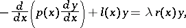 | (1) |
together with some boundary conditions, where  and
and  are positive,
  is real and
  is a complex parameter. Serious studies of this problem were started by J.Ch. Sturm and J. Liouville. The methods and notions that originated during studies of the Sturm–Liouville problem played an important role in the development of many directions in mathematics and physics. It was and remains a constant source of new ideas and problems in the spectral theory of operators and in related problems in analysis. Recently it gained even greater significance, when its relation to certain non-linear evolution equations of mathematical physics were discovered.
If  is differentiable and
  is twice differentiable, then, by a substitution, equation (1) can be reduced to (see [1])
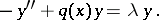 | (2) |
It is customary to distinguish between regular and singular problems. A Sturm–Liouville problem for equation (2) is called regular if the interval  in which
  varies is finite and if the function
  is summable on the entire interval
  . If the interval
  is infinite or if
  is not summable (or both), then the problem is called singular.
Below the following possibilities will be considered in some detail: 1) the interval  is finite (in this case, without loss of generality, one may assume
  and
and  ); 2)
); 2)  ,
,  ; or 3)
  ,
,  .
.
 . Consider the problem given on the interval
  by equation (2) and the separated boundary conditions
 | (3) |
where  is a real summable function on
  ,
,  and
and  are arbitrary finite or infinite fixed real numbers and
  is a complex parameter. If
 , then the first (second) condition in (3) is replaced by
 . To be specific it is further assumed that all numbers occurring in the boundary conditions are finite.
The number  is called an eigenvalue for the problem (2), (3) if for
  equation (2) has a non-trivial solution
  that satisfies (3); the function
  is then called the eigenfunction corresponding to the eigenvalue
  .
.
The eigenvalues for the boundary value problem (2), (3) are real; to the distinct eigenvalues correspond linearly independent eigenfunctions (since  and the numbers
  are real, the eigenfunctions for the problem (2), (3) can be chosen to be real); eigenfunctions
  and
and  corresponding to different eigenvalues are unique and orthogonal, i.e.
  .
.
There exists an unboundedly-increasing sequence of eigenvalues  for the boundary value problem (2), (3); moreover, the eigenfunction
  corresponding to the eigenvalue
  has precisely
  zeros in the interval
  .
.
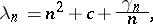
Let  be the Sobolev space of complex-valued functions on the interval
  that have
  absolutely-continuous derivatives and with
  -th derivatives summable on
  . If
. If 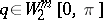 , then the eigenvalues
  of the boundary value problem (2), (3) for large
  satisfy the following asymptotic equation (see [4]):
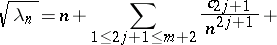 |
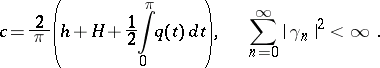
 |
where  are numbers independent of
  ,
,
 |
 |
 |
 does not depend on
  , and
, and
 |
The above implies, in particular, that if 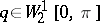 , then
 |
where
 |
Thus, the series 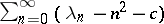 is convergent. Its sum is called the regularized trace of the problem (2), (3) (see [13]):
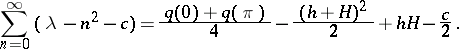 |
Let  be the orthonormal eigenfunctions of the problem (2), (3) corresponding to the eigenvalues
  . For any function
  the so-called Parseval equality holds:
 |
where
 |
and the following formula for eigenfunction expansion is valid:
 | (4) |
where the series converges in the metric of  . Completeness and expansion theorems for a regular Sturm–Liouville problem were first proved by V.A. Steklov [14].
If the function  has a continuous second derivative and satisfies the boundary conditions (3), then the following assertions hold (see [15]):
a) the series (4) converges absolutely and uniformly on  to
to  ;
;
b) the once-differentiated series (4) converges absolutely and uniformly on  to
to  ;
;
c) at any point where  satisfies some local condition of expansion in a Fourier series (e.g. is of bounded variation), the twice-differentiated series (4) converges to
  .
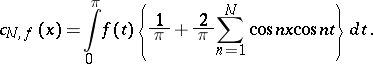
.
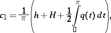
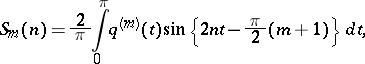
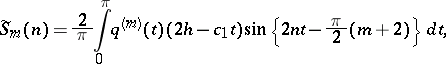
For any function  the series (4) is uniformly equiconvergent with the Fourier cosine series of
  , i.e.
 |
where
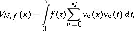 |
 |
This means that the expansion of  with respect to the eigenfunctions of the boundary value problem (2), (3) converges under the same conditions as the expansion of
  in a Fourier cosine series (see [1], [4]).
 . The differential equation (2) is considered on the half-line
  with a boundary condition at zero:
 | (5) |
The function  is assumed to be real and summable on any finite subinterval of
  and
and  is assumed to be real.
Let  be a solution of (2) with the initial conditions
  ,
,  (so that
  satisfies also the boundary condition (5)). Let
  be any function from
  and let
  , where
  is an arbitrary finite positive number. For any function
  and any number
  there is at least one decreasing function
  ,
,  , independent of
  , that has the following properties:
a) there is a function  , which is the limit of
  for
for  in the metric of
  (the space of
  -measurable functions
  for which
  ), i.e.
 |
b) the Parseval equality is valid:
 |
The function  is called the spectral function (or spectral density) for the boundary value problem (2), (5) (see [9]–[11]).
For the spectral function  of the problem (2), (5) the following asymptotic formula is true (see [16]) (for a more precise form, see ):
 |
 |
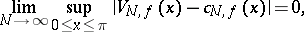
The following equiconvergence theorem is valid : For an arbitrary function  , let
, let
 |
 |
(the integrals converge in the metrics of  and
and  , respectively); then for any fixed
  the integral
 |
converges absolutely and uniformly with respect to  , and
, and
 |
 |
Let problem (2), (5) have a discrete spectrum, i.e. let its spectrum consist of a countable number of eigenvalues  with a unique limit point at infinity. Under certain restrictions on the function
  , for the function
  , i.e. the number of eigenvalues less than
  , the following asymptotic formula is valid:
 |
Simultaneously with  , a second solution
  of equation (2) is introduced, satisfying the conditions
  ,
,  , so that
  and
and  form a fundamental system of solutions of (2). For a fixed
 and
and  the following fractional-linear function is considered:
 |
When the independent variable  varies on the real line, the point
  describes a circle bounding a disc
  . It always lies in the same half-plane (lower or upper) as
  . When
  increases,
  shrinks, i.e. for
  the disc
  lies entirely inside the disc
  . There is (for
  ) a limit disc or a point
  ; if
; if
 | (6) |
then  is a disc, otherwise it is a point (see [10]). If condition (6) is fulfilled for some non-real value of
  , then it is fulfilled for all values of
  . In the case of a limit disc, for any value of
  all solutions of (2) belong to
  , and in the case of a limit point, for any non-real value of
  this equation has the solution
  , which belongs to
  , where
  is the limit point
  .
.
If  , where
  is some positive constant, then the case of a limit point holds (see [19]); for more general results see [20], [21].
 . Consider now equation (2) on the whole line
  under the assumption that
  is a real summable function on every finite subinterval of
  . Let
. Let  ,
,  be the solutions of (2) satisfying the conditions
  ,
,  .
.
There is at least one real symmetric non-decreasing matrix-function
 |
with the following properties:
a) for any function  there exist functions
  ,
,  , defined by
 |
where the limit is in the metric of  ;
;
b) the Parseval equality is valid:
 |
References
| [1] | B.M. Levitan, I.S. Sargsyan, "An introduction to spectral theory" , Amer. Math. Soc. (1975) (Translated from Russian) |
| [2] | B.M. Levitan, "Eigenfunction expansions of second-order differential equations" , Moscow-Leningrad (1950) (In Russian) |
| [3] | B.M. Levitan, "Generalized translation operators and some of their applications" , Israel Program Sci. Transl. (1964) (Translated from Russian) |
| [4] | V.A. Marchenko, "Sturm–Liouville operators and applications" , Birkhäuser (1986) (Translated from Russian) |
| [5] | E.C. Titchmarsh, "Eigenfunction expansions associated with second-order differential equations" , 1 , Clarendon Press (1962) |
| [6] | E.A. Coddington, N. Levinson, "Theory of ordinary differential equations" , McGraw-Hill (1955) pp. Chapts. 13–17 |
| [7] | M.A. Naimark, "Lineare Differentialoperatoren" , Akademie Verlag (1960) (Translated from Russian) |
| [8] | A.G. Kostyuchenko, I.S. Sargsyan, "Distribution of eigenvalues" , Moscow (1979) (In Russian) |
| [9] | H. Weyl, "Über gewöhnliche lineare Differentialgleichungen mit singulären Stellen und ihre Eigenfunktionen" Gött. Nachr. (1909) pp. 37–64 |
| [10] | H. Weyl, "Über gewöhnliche lineare Differentialgleichungen mit Singularitäten und die Zugehörigen Entwicklungen willküriger Funktionen" Math. Ann. , 68 (1910) pp. 220–269 |
| [11] | H. Weyl, "Über gewöhnliche lineare Differentialgleichungen mit singulären Stellen und ihre Eigenfunktionen (2)" Gött. Nachr. (1910) pp. 442–467 |
| [12] | M.G. Krein, "On the indeterminate case of the Sturm–Liouville boundary problem in the interval  " Izv. Akad. Nauk SSSR Ser. Mat. , 16 : 4 (1952) pp. 293–324 (In Russian) " Izv. Akad. Nauk SSSR Ser. Mat. , 16 : 4 (1952) pp. 293–324 (In Russian) |
| [13] | I.M. Gel'fand, B.M. Levitan, "On a simple identity for the characteristic values of a differential operator of the second order" Dokl. Akad. Nauk SSSR , 88 : 4 (1953) pp. 593–596 (In Russian) |
| [14] | V.A. Steklov, "On the development of a given function in a series made up from harmonic functions" Soobshch. Khar'k. Mat. Obshch. , 5 : 1–2 (1896) (In Russian) |
| [15] | B.M. Levitan, I.S. Sargsyan, "Some problems in the theory of the Sturm–Liouville equation" Russian Math. Surveys , 15 : 1 (1960) pp. 1–95 Uspekhi Mat. Nauk , 15 : 1 (1960) pp. 3–98 |
| [16] | V.A. Marchenko, "On the theory of a second-order differential operator" Dokl. Akad. Nauk SSSR , 72 : 3 (1950) pp. 457–460 (In Russian) |
| [17a] | B.M. Levitan, "On the asymptotic behaviour of the spectral function of a second-order self-adjoint differential equation, and on eigenfunction expansion" Izv. Akad. Nauk SSSR Ser. Mat. , 17 : 4 (1953) pp. 331–364 (In Russian) |
| [17b] | B.M. Levitan, "On the asymptotic behaviour of the spectral function of a second-order self-adjoint differential equation, and on eigenfunction expansion II" Izv. Akad. Nauk SSSR Ser. Mat. , 19 : 1 (1955) pp. 33–58 (In Russian) |
| [18] | J.S. de Wet, F. Mandl, "On the asymptotic distribution of eigenvalues" Proc. Roy. Soc. Ser. A , 200 (1950) pp. 572–580 |
| [19] | E. Titchmarsh, "On the uniqueness of the Green's function associated with a second-order differential equation" Canad. J. Math. , 1 (1949) pp. 191–198 |
| [20] | N. Levinson, "Criteria for the limit-point case for second order linear differential operators" Časopis Pěst Mat. Fys. , 74 (1949) pp. 17–20 |
| [21] | D. Sears, E. Titchmarsh, "Some eigenfunction formulae" Quart. J. Math. (Oxford Ser.) , 1 (1950) pp. 165–175 |
Comments
Eigenvalue problems of type (2) and the corresponding inverse problems (cf. Sturm–Liouville problem, inverse) play a major role in solving soliton equations, cf. Soliton, by the so-called "inverse-scattering methodinverse scattering method" . Cf. Korteweg–de Vries equation for a description of this method, and/or e.g. [a1]–[a5].
In the West one usually considers the boundary of  , and speaks of the limit point and limit circle cases.
References
| [a1] | P.D. Lax, "Integrals of nonlinear equations of evolution and solitary waves" Comm. Pure Appl. Math. , 21 (1968) pp. 467–490 |
| [a2] | V.E. Zakharov, A.B. Shabat, Soviet Phys. JETP (1972) pp. 62–69 |
| [a3] | R.M. Miura, "The Korteweg–de Vries equation: a survey of results" SIAM Review , 18 (1976) pp. 412–459 |
| [a4] | W. Eckhaus, A. van Harten, "The inverse scattering transformation and the theory of solitons" , North-Holland (1983) |
| [a5] | P.C. Schuur, "Asymptotic analysis of soliton problems" , Springer (1986) |
| [a6] | Yu.M. [Yu.M. Berezanskii] Berezanskiy, "Expansions in eigenfunctions of selfadjoint operators" , Amer. Math. Soc. (1968) (Translated from Russian) |
| [a7] | W.T. Reid, "Sturmian theory for ordinary differential equations" , Springer (1980) |
Sturm-Liouville problem. Encyclopedia of Mathematics. URL: http://encyclopediaofmath.org/index.php?title=Sturm-Liouville_problem&oldid=48885