Difference between revisions of "Statistical problems in the theory of stochastic processes"
(Importing text file) |
Ulf Rehmann (talk | contribs) m (MR/ZBL numbers added) |
||
| Line 8: | Line 8: | ||
===Example 1.=== | ===Example 1.=== | ||
| − | The process <img align="absmiddle" border="0" src="https://www.encyclopediaofmath.org/legacyimages/s/s087/s087450/s08745012.png" /> is either the sum of a non-random function <img align="absmiddle" border="0" src="https://www.encyclopediaofmath.org/legacyimages/s/s087/s087450/s08745013.png" /> (a | + | The process <img align="absmiddle" border="0" src="https://www.encyclopediaofmath.org/legacyimages/s/s087/s087450/s08745012.png" /> is either the sum of a non-random function <img align="absmiddle" border="0" src="https://www.encyclopediaofmath.org/legacyimages/s/s087/s087450/s08745013.png" /> (a "signal" ) and a random function <img align="absmiddle" border="0" src="https://www.encyclopediaofmath.org/legacyimages/s/s087/s087450/s08745014.png" /> (the "noise" ), or is a single random function <img align="absmiddle" border="0" src="https://www.encyclopediaofmath.org/legacyimages/s/s087/s087450/s08745015.png" />. The hypothesis <img align="absmiddle" border="0" src="https://www.encyclopediaofmath.org/legacyimages/s/s087/s087450/s08745016.png" />: <img align="absmiddle" border="0" src="https://www.encyclopediaofmath.org/legacyimages/s/s087/s087450/s08745017.png" /> must be tested against the alternative <img align="absmiddle" border="0" src="https://www.encyclopediaofmath.org/legacyimages/s/s087/s087450/s08745018.png" />: <img align="absmiddle" border="0" src="https://www.encyclopediaofmath.org/legacyimages/s/s087/s087450/s08745019.png" /> (the problem of locating a signal in noise). This is an example of testing a statistical hypothesis. |
===Example 2.=== | ===Example 2.=== | ||
| Line 28: | Line 28: | ||
<table class="eq" style="width:100%;"> <tr><td valign="top" style="width:94%;text-align:center;"><img align="absmiddle" border="0" src="https://www.encyclopediaofmath.org/legacyimages/s/s087/s087450/s08745050.png" /></td> </tr></table> | <table class="eq" style="width:100%;"> <tr><td valign="top" style="width:94%;text-align:center;"><img align="absmiddle" border="0" src="https://www.encyclopediaofmath.org/legacyimages/s/s087/s087450/s08745050.png" /></td> </tr></table> | ||
| − | In this case <img align="absmiddle" border="0" src="https://www.encyclopediaofmath.org/legacyimages/s/s087/s087450/s08745051.png" /> does not exist. The singularity of the measures <img align="absmiddle" border="0" src="https://www.encyclopediaofmath.org/legacyimages/s/s087/s087450/s08745052.png" /> leads to important and somewhat paradoxical statistical results, allowing for error-free inferences concerning the parameter <img align="absmiddle" border="0" src="https://www.encyclopediaofmath.org/legacyimages/s/s087/s087450/s08745053.png" />. For example, let <img align="absmiddle" border="0" src="https://www.encyclopediaofmath.org/legacyimages/s/s087/s087450/s08745054.png" />; the singularity of the measures <img align="absmiddle" border="0" src="https://www.encyclopediaofmath.org/legacyimages/s/s087/s087450/s08745055.png" /> and <img align="absmiddle" border="0" src="https://www.encyclopediaofmath.org/legacyimages/s/s087/s087450/s08745056.png" /> means that, using the test | + | In this case <img align="absmiddle" border="0" src="https://www.encyclopediaofmath.org/legacyimages/s/s087/s087450/s08745051.png" /> does not exist. The singularity of the measures <img align="absmiddle" border="0" src="https://www.encyclopediaofmath.org/legacyimages/s/s087/s087450/s08745052.png" /> leads to important and somewhat paradoxical statistical results, allowing for error-free inferences concerning the parameter <img align="absmiddle" border="0" src="https://www.encyclopediaofmath.org/legacyimages/s/s087/s087450/s08745053.png" />. For example, let <img align="absmiddle" border="0" src="https://www.encyclopediaofmath.org/legacyimages/s/s087/s087450/s08745054.png" />; the singularity of the measures <img align="absmiddle" border="0" src="https://www.encyclopediaofmath.org/legacyimages/s/s087/s087450/s08745055.png" /> and <img align="absmiddle" border="0" src="https://www.encyclopediaofmath.org/legacyimages/s/s087/s087450/s08745056.png" /> means that, using the test "accept H0 if x A, reject H0 if x A" , the hypotheses <img align="absmiddle" border="0" src="https://www.encyclopediaofmath.org/legacyimages/s/s087/s087450/s08745057.png" />: <img align="absmiddle" border="0" src="https://www.encyclopediaofmath.org/legacyimages/s/s087/s087450/s08745058.png" /> and <img align="absmiddle" border="0" src="https://www.encyclopediaofmath.org/legacyimages/s/s087/s087450/s08745059.png" />: <img align="absmiddle" border="0" src="https://www.encyclopediaofmath.org/legacyimages/s/s087/s087450/s08745060.png" /> are distinguished error-free. The presence of such perfect tests often demonstrates that the statistical problem is not posed entirely satisfactorily and that certain essential random disturbances are excluded from it. |
===Example 3.=== | ===Example 3.=== | ||
| Line 105: | Line 105: | ||
The problem of estimating <img align="absmiddle" border="0" src="https://www.encyclopediaofmath.org/legacyimages/s/s087/s087450/s087450167.png" /> when <img align="absmiddle" border="0" src="https://www.encyclopediaofmath.org/legacyimages/s/s087/s087450/s087450168.png" /> is known is often treated as a linear problem. This group of problems also includes the more general problems of estimating regression coefficients through observations of the form (*) with stationary <img align="absmiddle" border="0" src="https://www.encyclopediaofmath.org/legacyimages/s/s087/s087450/s087450169.png" />. | The problem of estimating <img align="absmiddle" border="0" src="https://www.encyclopediaofmath.org/legacyimages/s/s087/s087450/s087450167.png" /> when <img align="absmiddle" border="0" src="https://www.encyclopediaofmath.org/legacyimages/s/s087/s087450/s087450168.png" /> is known is often treated as a linear problem. This group of problems also includes the more general problems of estimating regression coefficients through observations of the form (*) with stationary <img align="absmiddle" border="0" src="https://www.encyclopediaofmath.org/legacyimages/s/s087/s087450/s087450169.png" />. | ||
| − | Let <img align="absmiddle" border="0" src="https://www.encyclopediaofmath.org/legacyimages/s/s087/s087450/s087450170.png" /> have zero mean and spectral density <img align="absmiddle" border="0" src="https://www.encyclopediaofmath.org/legacyimages/s/s087/s087450/s087450171.png" /> depending on a finite-dimensional parameter <img align="absmiddle" border="0" src="https://www.encyclopediaofmath.org/legacyimages/s/s087/s087450/s087450172.png" />. If the process <img align="absmiddle" border="0" src="https://www.encyclopediaofmath.org/legacyimages/s/s087/s087450/s087450173.png" /> is Gaussian, formulas can be derived for the likelihood ratio <img align="absmiddle" border="0" src="https://www.encyclopediaofmath.org/legacyimages/s/s087/s087450/s087450174.png" /> (if the ratio exists), which in a number of cases make it possible to find maximum-likelihood estimators or | + | Let <img align="absmiddle" border="0" src="https://www.encyclopediaofmath.org/legacyimages/s/s087/s087450/s087450170.png" /> have zero mean and spectral density <img align="absmiddle" border="0" src="https://www.encyclopediaofmath.org/legacyimages/s/s087/s087450/s087450171.png" /> depending on a finite-dimensional parameter <img align="absmiddle" border="0" src="https://www.encyclopediaofmath.org/legacyimages/s/s087/s087450/s087450172.png" />. If the process <img align="absmiddle" border="0" src="https://www.encyclopediaofmath.org/legacyimages/s/s087/s087450/s087450173.png" /> is Gaussian, formulas can be derived for the likelihood ratio <img align="absmiddle" border="0" src="https://www.encyclopediaofmath.org/legacyimages/s/s087/s087450/s087450174.png" /> (if the ratio exists), which in a number of cases make it possible to find maximum-likelihood estimators or "good" approximations of them (for large <img align="absmiddle" border="0" src="https://www.encyclopediaofmath.org/legacyimages/s/s087/s087450/s087450175.png" />). Under sufficiently broad assumptions these estimators are asymptotically normal <img align="absmiddle" border="0" src="https://www.encyclopediaofmath.org/legacyimages/s/s087/s087450/s087450176.png" /> and asymptotically efficient. |
===Example 7.=== | ===Example 7.=== | ||
| Line 215: | Line 215: | ||
====References==== | ====References==== | ||
| − | <table><TR><TD valign="top">[1]</TD> <TD valign="top"> | + | <table><TR><TD valign="top">[1]</TD> <TD valign="top"> U. Grenander, "Stochastic processes and statistical inference" ''Ark. Mat.'' , '''1''' (1950) pp. 195–277 {{MR|0039202}} {{ZBL|0058.35501}} {{ZBL|0041.45807}} </TD></TR><TR><TD valign="top">[2]</TD> <TD valign="top"> E.J. Hannan, "Time series analysis" , Methuen , London (1960) {{MR|0114281}} {{ZBL|0095.13204}} </TD></TR><TR><TD valign="top">[3]</TD> <TD valign="top"> U. Grenander, M. Rosenblatt, "Statistical analysis of stationary time series" , Wiley (1957) {{MR|0084975}} {{ZBL|0080.12904}} </TD></TR><TR><TD valign="top">[4]</TD> <TD valign="top"> U. Grenander, "Abstract inference" , Wiley (1981) {{MR|0599175}} {{ZBL|0505.62069}} </TD></TR><TR><TD valign="top">[5]</TD> <TD valign="top"> Yu.A. Rozanov, "Infinite-dimensional Gaussian distributions" ''Proc. Steklov Inst. Math.'' , '''108''' (1971) ''Trudy Mat. Inst. Steklov.'' , '''108''' (1968) {{MR|0436304}} {{ZBL|}} </TD></TR><TR><TD valign="top">[6]</TD> <TD valign="top"> I.A. Ibragimov, Yu.A. Rozanov, "Gaussian random processes" , Springer (1978) (Translated from Russian) {{MR|0543837}} {{ZBL|0392.60037}} </TD></TR><TR><TD valign="top">[7]</TD> <TD valign="top"> D.R. Brillinger, "Time series. Data analysis and theory" , Holt, Rinehart & Winston (1975) {{MR|0443257}} {{ZBL|0321.62004}} </TD></TR><TR><TD valign="top">[8]</TD> <TD valign="top"> P. Billingsley, "Statistical inference for Markov processes" , Univ. Chicago Press (1961) {{MR|1531450}} {{MR|0123419}} {{ZBL|0106.34201}} </TD></TR><TR><TD valign="top">[9]</TD> <TD valign="top"> R.S. Liptser, A.N. Shiryaev, "Statistics of random processes" , '''1–2''' , Springer (1977–1978) (Translated from Russian) {{MR|1800858}} {{MR|1800857}} {{MR|0608221}} {{MR|0488267}} {{MR|0474486}} {{ZBL|1008.62073}} {{ZBL|1008.62072}} {{ZBL|0556.60003}} {{ZBL|0369.60001}} {{ZBL|0364.60004}} </TD></TR><TR><TD valign="top">[10]</TD> <TD valign="top"> A.M. Yaglom, "Correlation theory of stationary and related random functions" , '''1–2''' , Springer (1987) (Translated from Russian) {{MR|0915557}} {{MR|0893393}} {{ZBL|0685.62078}} {{ZBL|0685.62077}} </TD></TR><TR><TD valign="top">[11]</TD> <TD valign="top"> T.M. Anderson, "The statistical analysis of time series" , Wiley (1971) {{MR|0283939}} {{ZBL|0225.62108}} </TD></TR></table> |
Revision as of 17:35, 31 March 2012
A branch of mathematical statistics devoted to statistical inferences on the basis of observations represented as a random process. In the most common formulation, the values of a random function  for
for  are observed, and on the basis of these observations statistical inferences must be made regarding certain characteristics of
  . Such a broad definition also formally includes all the classical statistics of independent observations. In fact, statistics of random processes is often taken to mean only the statistics of dependent observations, excluding the statistical analysis of a large number of independent realizations of a random process. Here the foundations of the statistical theory, the basic formulations of problems (cf. Statistical estimation; Statistical hypotheses, verification of), the basic concepts (sufficiency, unbiasedness, consistency, etc.) are the same as in the classical theory. However, when solving concrete problems, significant difficulties and phenomena of a new type arise from time to time. These difficulties are partially caused by the fact of dependence and the more complex structure of the process under consideration, and partially, in the case of observations in continuous time, by the need to examine distributions in infinite-dimensional spaces.
In fact, when solving statistical problems in the theory of random processes, the structure of the process under consideration is crucial, while when classifying random processes, statistical problems of Gaussian, Markov, stationary, branching, diffusion, and other processes are studied. Of these, the most far-reaching is the statistical theory of stationary processes (time-series analysis).
The need for a statistical analysis of random processes arose in the 19th century in the form of analysis of meteorological and economic series and studies on cyclic processes (price fluctuation, sun spots). In modern times, the number of problems covered by the statistical analysis of random processes has become extraordinarily large. To cite but a few examples, statistical analysis of random noise, vibrations, turbulence, wave motion in a sea, cardiograms and encephalograms, etc. The theoretical aspects of extracting a signal from a background of noise can be seen to a significant degree as a statistical problem in the theory of random processes.
Below it is proposed that a segment  ,
,  , of the random process
  be observed, whereby the parameter
  passes either through the whole interval
  , or through the integers in this interval. In statistical problems, the distribution
  of the process
  is usually known only to belong to some family of distributions
  . This family can always be written in parametric form.
Example 1.
The process  is either the sum of a non-random function
  (a "signal" ) and a random function
  (the "noise" ), or is a single random function
  . The hypothesis
  :
:  must be tested against the alternative
  :
:  (the problem of locating a signal in noise). This is an example of testing a statistical hypothesis.
Example 2.
The process  , where
  is an unknown non-random function (the signal), while
  is a random process (the noise). The function
  , or its value
  at a given point
  , has to be estimated. Similarly, it can be proposed that
  , where
  is a known function, depending on an unknown parameter
  , which must also be estimated through the observation of
  (problems of extracting a signal from a background of noise). These are examples of estimation problems.
The likelihood ratio for random processes.
In statistical problems, likelihood ratios and likelihood functions play an important role (see Neyman–Pearson lemma; Statistical hypotheses, verification of; Statistical estimation). The likelihood ratio of two distributions  and
and  is the density
 |
The likelihood function is the function
 |
where  is a
is a  -finite measure relative to which all measures
  are absolutely continuous. In the discrete case, where
  runs through the integers of
  and
and  , the likelihood ratio always exists if the distributions
  and
and  have positive densities, and it coincides with the ratio of these two densities.
If  runs through the entire interval
  , then cases may arise in which the measures
  and
and  are not absolutely continuous with respect to each other; moreover, situations can arise in which
  and
and  are mutually singular, i.e. where for a set
  in the space of realizations of
  ,
,
 |
In this case  does not exist. The singularity of the measures
  leads to important and somewhat paradoxical statistical results, allowing for error-free inferences concerning the parameter
  . For example, let
  ; the singularity of the measures
  and
and  means that, using the test "accept H0 if x A, reject H0 if x A" , the hypotheses
  :
:  and
and  :
:  are distinguished error-free. The presence of such perfect tests often demonstrates that the statistical problem is not posed entirely satisfactorily and that certain essential random disturbances are excluded from it.
Example 3.
Let  , where
  is a stationary ergodic process with zero average and
  is a real parameter. Let the realizations of
  with probability 1 be analytic in a strip containing the real axis. According to the ergodic theorem,
 |
and all measures  are also mutually singular. Since an analytic function
  is completely defined by its values in a neighbourhood of zero, the parameter
  is error-free when estimated through the observations
  for any
  .
.
The calculation of the likelihood ratio in those cases where it exists is a difficult problem. Calculations are often based on the limit relation
 |
where  are the densities of the vector
  , while
  is a dense set in
  . Study of the right-hand side of the above equality also is useful in investigating the possible singularity of
  and
and  .
.
Example 4.
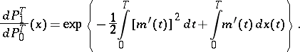
Suppose one has either the observation  , where
  is a Wiener process (hypothesis
  ), or
), or  , where
  is a non-random function (hypothesis
  ). The measures
  are mutually absolutely continuous if
  , and mutually singular if
  . The likelihood ratio equals
 |
Example 5.
Let  , where
  is a real parameter and
  is a stationary Gaussian Markov process with mean zero and known correlation function
  ,
,  . The measures
  are mutually absolutely continuous with likelihood function
 |
 |
In particular,  is a sufficient statistic for the family
  .
.
Linear problems in the statistics of random processes.
Let the function
 | (*) |
be observed, where  is a random process with mean zero and known correlation function
  ,
,  are known non-random functions,
  is an unknown parameter (
 are the regression coefficients), and the parameter set
  is a subset of
  . Linear estimators for
  are estimators of the form
  , or their limits in the mean square. The problem of finding optimal unbiased linear estimators in the mean square reduces to the solution of linear algebraic or linear integral equations in
  . Indeed, an optimal estimator
  is defined by the equations
  for any
  of the form
  ,
,  . In a number of cases, estimators of
  , obtained asymptotically by the method of least squares, when
  , are not worse than the optimal linear estimators. Estimators obtained by the method of least squares are calculated more simply and do not depend on
  .
.
Example 6.
Under the conditions of example 5,  ,
,  . The optimal unbiased linear estimator takes the form
 |
The estimator
 |
has asymptotically the same variance.
Statistical problems of Gaussian processes.
Let  be a Gaussian process for all
  . For Gaussian processes one has the alternatives: Any two measures
  are either mutually absolutely continuous or are singular. Since the Gaussian distribution
  is completely defined by the mean value
  and the correlation function
  , the likelihood ratio
  is expressed in terms of
  ,
,  ,
,  ,
,  in a complex way. The case where
  , and
, and  a continuous function, is relatively simple. Let
  ,
,  ; let
; let  , and
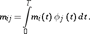
, and  , be the eigenvalues, and the corresponding normalized eigenfunctions in
  , of the integral equation
 |
let the means  and
and  be continuous functions; and let
 |
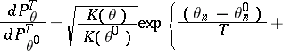
The measures  are absolutely continuous if and only if
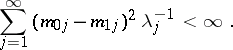 |
Here,
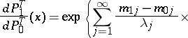 |
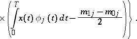 |
This equality can be used to devise a test for the hypothesis  :
:  against the alternative
  :
:  under the assumption that the function
  is known to the observer.
Statistical problems of stationary processes.
Let the observation  be a stationary process with mean
  and correlation function
  ; let
; let  and
and  be its spectral density and spectral function, respectively. The basic problems of the statistics of stationary processes relate to hypotheses testing and to estimating the characteristics
  ,
,  ,
,  ,
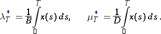
,  . In the case of an ergodic process
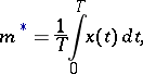
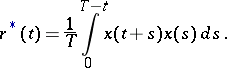
  , consistent estimators (when
  ) for
) for  and
and  , respectively, are provided by
 |
 |
The problem of estimating  when
when  is known is often treated as a linear problem. This group of problems also includes the more general problems of estimating regression coefficients through observations of the form (*) with stationary
  .
.
Let  have zero mean and spectral density
  depending on a finite-dimensional parameter
  . If the process
  is Gaussian, formulas can be derived for the likelihood ratio
  (if the ratio exists), which in a number of cases make it possible to find maximum-likelihood estimators or "good" approximations of them (for large
  ). Under sufficiently broad assumptions these estimators are asymptotically normal
  and asymptotically efficient.
Example 7.
Let  be a stationary Gaussian process in continuous time with rational spectral density
 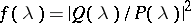 , where
  and
and  are polynomials. The measures
  corresponding to the rational spectral densities
  are absolutely continuous if and only if
 |
Here the parameter  is the set of all coefficients of the polynomials
  .
.
Example 8.
An important class of stationary Gaussian processes consists of the auto-regressive processes (cf. Auto-regressive process)  :
:
 |
where  is a Gaussian white noise of unit intensity and
  is an unknown parameter. In this case the spectral density is
 |
where
 |
The likelihood function is
 |
 |
 |
Here,  and
and  are quadratic forms in
  , depending on the values
  ,
,  , at the points
  , and
, and  is the determinant of the correlation matrix of the vector
  .
.
Maximum-likelihood estimators for the auto-regression parameter  are asymptotically normal and asymptotically efficient. These properties are shared by the solution
  of the approximate likelihood equation
 |
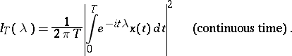
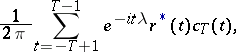
An important role in statistical studies on the spectrum of a stationary process is played by the periodogram  . This statistic is defined as
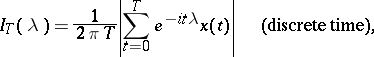 |
 |
The periodogram is widely used in constructing different kinds of estimators for  ,
,  and criteria for testing hypotheses on these characteristics. Under broad assumptions, the statistics
 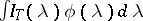 are consistent estimators for
 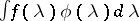 . In particular,
  may serve as an estimator for
  . If the sequence
  converges in an appropriate way to the
  -function
  , then the integrals
  will be consistent estimators for
  . Functions of the form
  ,
,  , are often used in the capacity of the functions
  . If
. If  is a process in discrete time, these estimators can be written in the form
 |
where the empirical correlation function is
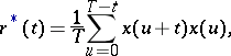 |
while the non-random coefficients  are defined by the choice of
  and
and  . This choice, in turn, depends on a priori information on
  . A similar representation also holds for processes in continuous time.
Problems in the statistical analysis of stationary processes sometimes also include problems of extrapolation, interpolation and filtration of stationary processes.
Statistical problems of Markov processes.
Let the observations  belong to a homogeneous Markov chain. Under sufficiently broad assumptions the likelihood function is
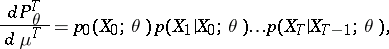 |
where  ,
,  are the initial and transition densities of the distribution. This expression is similar to the likelihood function for a sequence of independent observations, and when the regularity conditions are observed (smoothness in
  ), a theory can be constructed for hypotheses testing and estimation which is analogous to the corresponding theory for independent observations.
A more complex situation arises if  is a Markov process in continuous time. Let
  be a homogeneous Markov process with a finite number of states
  and differentiable transition probabilities
  . The transition probability matrix is defined by the matrix
  ,
,  ,
,  . Let
. Let  be independent of
  at the initial time. By choosing any matrix
  , one finds
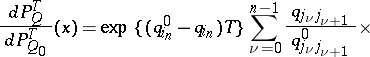 |
 |
Here the statistics  ,
,  ,
,  are defined in the following way:
  is the number of jumps of
  on the interval
  ;
;  is the moment of the
  -th jump,
  , and
, and  . It follows that the maximum-likelihood estimators for the parameters
  are:
are:  , where
  is the number of transitions from
  to
to  on
on  , while
  is the time spent by the process
  in the state
  .
.
Example 9.
Let  be a birth-and-death process with constant intensities of birth
  and death
  . This means that
  ,
,  ,
,  , and
, and  if
if  . In this example the number of states is infinite. Let
  . The likelihood ratio is
 |
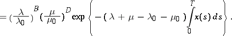 |
Here  is the total number of births (jumps of measure
  ) and
) and  is the number of deaths (jumps of measure
  ). Maximum-likelihood estimators for
  and
and  are
are
 |
Let  be a diffusion process with drift coefficient
  and diffusion coefficient
  , such that
  satisfies the stochastic differential equation
 |
where  is a Wiener process. Then, under specific restrictions,
 |
 |
(here  is a fixed coefficient).
Example 10.
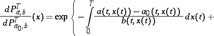
Let
 |
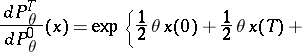
where  is a known function and
  is an unknown real parameter. If Wiener measure is denoted by
  , then the likelihood function is
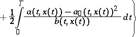
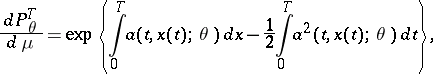 |
and, under regularity conditions, the Cramér–Rao inequality is satisfied: For an estimator  with bias
 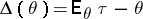 ,
,
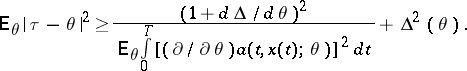 |
If the dependence on  is linear, the maximum-likelihood estimator is
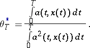 |
References
| [1] | U. Grenander, "Stochastic processes and statistical inference" Ark. Mat. , 1 (1950) pp. 195–277 MR0039202 Zbl 0058.35501 Zbl 0041.45807 |
| [2] | E.J. Hannan, "Time series analysis" , Methuen , London (1960) MR0114281 Zbl 0095.13204 |
| [3] | U. Grenander, M. Rosenblatt, "Statistical analysis of stationary time series" , Wiley (1957) MR0084975 Zbl 0080.12904 |
| [4] | U. Grenander, "Abstract inference" , Wiley (1981) MR0599175 Zbl 0505.62069 |
| [5] | Yu.A. Rozanov, "Infinite-dimensional Gaussian distributions" Proc. Steklov Inst. Math. , 108 (1971) Trudy Mat. Inst. Steklov. , 108 (1968) MR0436304 |
| [6] | I.A. Ibragimov, Yu.A. Rozanov, "Gaussian random processes" , Springer (1978) (Translated from Russian) MR0543837 Zbl 0392.60037 |
| [7] | D.R. Brillinger, "Time series. Data analysis and theory" , Holt, Rinehart & Winston (1975) MR0443257 Zbl 0321.62004 |
| [8] | P. Billingsley, "Statistical inference for Markov processes" , Univ. Chicago Press (1961) MR1531450 MR0123419 Zbl 0106.34201 |
| [9] | R.S. Liptser, A.N. Shiryaev, "Statistics of random processes" , 1–2 , Springer (1977–1978) (Translated from Russian) MR1800858 MR1800857 MR0608221 MR0488267 MR0474486 Zbl 1008.62073 Zbl 1008.62072 Zbl 0556.60003 Zbl 0369.60001 Zbl 0364.60004 |
| [10] | A.M. Yaglom, "Correlation theory of stationary and related random functions" , 1–2 , Springer (1987) (Translated from Russian) MR0915557 MR0893393 Zbl 0685.62078 Zbl 0685.62077 |
| [11] | T.M. Anderson, "The statistical analysis of time series" , Wiley (1971) MR0283939 Zbl 0225.62108 |
Statistical problems in the theory of stochastic processes. Encyclopedia of Mathematics. URL: http://encyclopediaofmath.org/index.php?title=Statistical_problems_in_the_theory_of_stochastic_processes&oldid=13453