Statistical estimation
One of the fundamental parts of mathematical statistics, dedicated to the estimation using random observations of various characteristics of their distribution.
Example 1.
Let  be independent random variables (or observations) with a common unknown distribution
  on the straight line. The empirical (sample) distribution
  which ascribes the weight
  to every random point
  is a statistical estimator for
  . The empirical moments
 |
serve as estimators for the moments  . In particular,
 |
is an estimator for the mean, and
 |
is an estimator for the variance.
Basic concepts.
In the general theory of estimation, an observation of  is a random element with values in a measurable space
  , whose unknown distribution belongs to a given family of distributions
  . The family of distributions can always be parametrized and written in the form
  . Here the form of dependence on the parameter and the set
  are assumed to be known. The problem of estimation using an observation
  of an unknown parameter
  or of the value
  of a function
  at the point
  consists of constructing a function
  from the observations made, which gives a sufficiently good approximation of
 .
.
A comparison of estimators is carried out in the following way. Let a non-negative loss function  be defined on
 , the sense of this being that the use of
  for the actual value of
  leads to losses
  . The mean losses and the risk function
  are taken as a measure of the quality of the statistic
  as an estimator of
  given the loss function
  . A partial order relation is thereby introduced on the set of estimators: An estimator
  is preferable to an estimator
  if
if  . In particular, an estimator
  of the parameter
  is said to be inadmissible (in relation to the loss function
  ) if an estimator
  exists such that
  for all
  , and for some
  strict inequality occurs. In this method of comparing the quality of estimators, many estimators prove to be incomparable, and, moreover, the choice of a loss function is to a large extent arbitrary.
It is sometimes possible to find estimators that are optimal within a certain narrower class of estimators. Unbiased estimators form an important class. If the initial experiment is invariant relative to a certain group of transformations, it is natural to restrict to estimators that do not disrupt the symmetry of the problem (see Equivariant estimator).
Estimators can be compared by their behaviour at "worst" points: An estimator  of
of  is called a minimax estimator relative to the loss function
  if
if
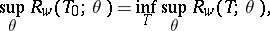 |
where the lower bound is taken over all estimators  .
.
In the Bayesian formulation of the problem (cf. Bayesian approach), the unknown parameter is considered to represent values of the random variable with a priori distribution  on
on  . In this case, the best estimator
  relative to the loss function
  is defined by the relation
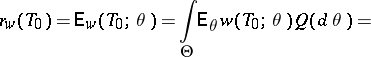 |
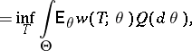 |
and the lower bound is taken over all estimators  .
.
There is a distinction between parametric estimation problems, in which  is a subset of a finite-dimensional Euclidean space, and non-parametric problems. In parametric problems one usually considers loss functions in the form
  , where
  is a non-negative, non-decreasing function on
  . The most frequently used quadratic loss function
  plays an important part.
If  is a sufficient statistic for the family
  , then it is often possible to restrict to estimators
  . Thus, if
  ,
,  , where
  is a convex function and
  is any estimator for
  , an estimator
  exists that is not worse than
  ; if
; if  is unbiased,
  can also be chosen unbiased (Blackwell's theorem). If
  is a complete sufficient statistic for the family
  and
and  is an unbiased estimator for
  , then an unbiased estimator in the form
  with minimum variance in the class of unbiased estimators exists (the Lehmann–Scheffé theorem).
As a rule, it is assumed that in parametric estimation problems the elements of the family  are absolutely continuous with respect to a certain
  -finite measure
  and that the density
 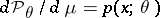 exists. If
  is a sufficiently-smooth function of
  and the Fisher information matrix
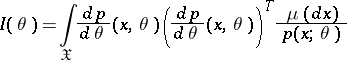 |
exists, the estimation problem is said to be regular. For regular problems, the accuracy of the estimation is bounded from below by the Cramér–Rao inequality: If  , then for any estimator
  ,
,
 |
Examples of estimation problems 2.
The most widespread formulation is that in which a sample of size  is observed:
  are independent identically-distributed variables taking values in a measurable space
  with common distribution density
  relative to a measure
  , and
, and  . In regular problems, if
  is the Fisher information on one observation, then the Fisher information of the whole sample
 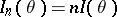 . The Cramér–Rao inequality takes the form
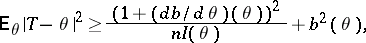 |
 |
 . Let
. Let  be normal random variables with distribution density
 |
Let the unknown parameter be  ;
;  and
and  can serve as estimators for
  and
and  , and
, and  is then a sufficient statistic. The estimator
  is unbiased, while
  is biased. If
  is known,
  is an unbiased estimator of minimal variance, and is a minimax estimator relative to the quadratic loss function.
 . Let
. Let  be normal random variables in
  with density
 |
The statistic  is an unbiased estimator of
  ; if
; if  , it is admissible relative to the quadratic loss function, if
  , it is inadmissible.
 . Let
. Let  be random variables in
  with unknown distribution density
  belonging to a given family
  of densities. For a sufficiently broad class
  , this is a non-parametric problem. The problem of estimating
  at a point
  is a problem of estimating the functional
  .
.
Example 3.
The linear regression model. The variables
 |
are observed; the  are random disturbances,
  ; the matrix
  is known; and the parameter
  must be estimated.
Example 4.
A segment of a stationary Gaussian process  ,
,  , with rational spectral density
  is observed; the unknown parameters
  ,
,  are to be estimated.
Methods of producing estimators.
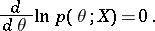
The most widely used maximum-likelihood method recommends that the estimator  defined as the maximum point of the random function
  is taken, the so-called maximum-likelihood estimator. If
  , the maximum-likelihood estimators are to be found among the roots of the likelihood equation
 |
In example 3, the method of least squares (cf. Least squares, method of) recommends that the minimum point of the function
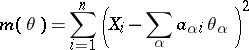 |
be used as the estimator.
Another method is to take a Bayesian estimator  relative to a loss function
  and an a priori distribution
  , although the initial formulation is not Bayesian. For example, if
  , it is possible to estimate
  by means of
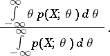 |
This is a Bayesian estimator relative to the quadratic loss function and a uniform a priori distribution.
The method of moments (cf. Moments, method of (in probability theory)) consists of the following. Let  , and suppose that there are
  "good" estimators
  for
for  . Estimators by the method of moments are solutions of the system
  . Empirical moments are frequently chosen in the capacity of
  (see example 1).
If the sample  is observed, then (see example 1) as an estimator for
  it is possible to choose
  . If the function
  is not defined (for example,
  , where
  is Lebesgue measure), appropriate modifications
  are chosen. For example, for an estimator of the density a histogram or an estimator of the form
 |
is used.
Asymptotic behaviour of estimators.
For the sake of being explicit a problem such as Example 2 is examined, in which  . It is to be expected that when
  , "good" estimators will get infinitely close to the characteristic being estimated. A sequence of estimators
  is called a consistent sequence of estimators of
  if
if  in the probability
  for all
  . The above methods of producing estimators lead, under broad hypotheses, to consistent estimators (cf. Consistent estimator). The estimators in example 1 are consistent. For regular estimation problems, maximum-likelihood estimators and Bayesian estimators are asymptotically normal with mean
  and correlation matrix
  . Under such conditions, these estimators are asymptotically locally minimax relative to a broad class of loss functions, and they can be considered as being asymptotically optimal (see Asymptotically-efficient estimator).
Interval estimation.
A random subset  of the set
  is called a confidence region for the estimator
  with confidence coefficient
  if
if  (
( ). Many confidence regions with a given
  usually exist, and the problem is to choose the one possessing certain optimal properties (for example, the interval of minimum length, if
  ). Under the conditions of example 2.1, let
  . Then the interval
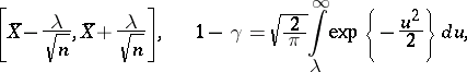 |
is a confidence interval with confidence coefficient  (see Interval estimator).
References
| [1] | R.A. Fisher, "On the mathematical foundations of theoretical statistics" Phil. Trans. Roy. Soc. London Ser. A , 222 (1922) pp. 309–368 |
| [2] | A.N. Kolmogorov, "Sur l'estimation statistique des paramètres de la loi de Gauss" Izv. Akad. Nauk SSSR Ser. Mat. , 6 : 1 (1942) pp. 3–32 |
| [3] | H. Cramér, "Mathematical methods of statistics" , Princeton Univ. Press (1946) |
| [4] | M.G. Kendall, A. Stuart, "The advanced theory of statistics" , 2. Inference and relationship , Griffin (1979) |
| [5] | I.A. Ibragimov, R.Z. [R.Z. Khas'minskii] Has'minskii, "Statistical estimation: asymptotic theory" , Springer (1981) (Translated from Russian) |
| [6] | N.N. Chentsov, "Statistical decision laws and optimal inference" , Amer. Math. Soc. (1982) (Translated from Russian) |
| [7] | S. Zacks, "The theory of statistical inference" , Wiley (1975) |
| [8] | U. Grenander, "Abstract inference" , Wiley (1981) |
Comments
References
| [a1] | E.L. Lehmann, "Theory of point estimation" , Wiley (1986) |
Statistical estimation. Encyclopedia of Mathematics. URL: http://encyclopediaofmath.org/index.php?title=Statistical_estimation&oldid=18593