Difference between revisions of "Riccati equation"
Ulf Rehmann (talk | contribs) m (tex encoded by computer) |
Ulf Rehmann (talk | contribs) m (Undo revision 48535 by Ulf Rehmann (talk)) Tag: Undo |
||
| Line 1: | Line 1: | ||
| − | |||
| − | |||
| − | |||
| − | |||
| − | |||
| − | |||
| − | |||
| − | |||
| − | |||
| − | |||
| − | |||
| − | |||
A first-order ordinary differential equation of the form | A first-order ordinary differential equation of the form | ||
| − | + | <table class="eq" style="width:100%;"> <tr><td valign="top" style="width:94%;text-align:center;"><img align="absmiddle" border="0" src="https://www.encyclopediaofmath.org/legacyimages/r/r081/r081770/r0817701.png" /></td> <td valign="top" style="width:5%;text-align:right;">(1)</td></tr></table> | |
| − | |||
| − | |||
| − | where | + | where <img align="absmiddle" border="0" src="https://www.encyclopediaofmath.org/legacyimages/r/r081/r081770/r0817702.png" />, <img align="absmiddle" border="0" src="https://www.encyclopediaofmath.org/legacyimages/r/r081/r081770/r0817703.png" /> and <img align="absmiddle" border="0" src="https://www.encyclopediaofmath.org/legacyimages/r/r081/r081770/r0817704.png" /> are constants. This equation was first studied by J. Riccati (1723, see [[#References|[1]]]); individual cases of the equation were examined earlier. D. Bernoulli (1724–1725) established that the equation (1) can be integrated by elementary functions if <img align="absmiddle" border="0" src="https://www.encyclopediaofmath.org/legacyimages/r/r081/r081770/r0817705.png" /> or <img align="absmiddle" border="0" src="https://www.encyclopediaofmath.org/legacyimages/r/r081/r081770/r0817706.png" />, where <img align="absmiddle" border="0" src="https://www.encyclopediaofmath.org/legacyimages/r/r081/r081770/r0817707.png" /> is an integer. J. Liouville (1841) proved that for other values of <img align="absmiddle" border="0" src="https://www.encyclopediaofmath.org/legacyimages/r/r081/r081770/r0817708.png" /> the solution of (1) cannot be expressed in quadratures by elementary functions. The general solution of (1) can be written with the aid of [[Cylinder functions|cylinder functions]] (see [[#References|[1]]]). |
| − | |||
| − | and | ||
| − | are constants. This equation was first studied by J. Riccati (1723, see [[#References|[1]]]); individual cases of the equation were examined earlier. D. Bernoulli (1724–1725) established that the equation (1) can be integrated by elementary functions if | ||
| − | or | ||
| − | where | ||
| − | is an integer. J. Liouville (1841) proved that for other values of | ||
| − | the solution of (1) cannot be expressed in quadratures by elementary functions. The general solution of (1) can be written with the aid of [[Cylinder functions|cylinder functions]] (see [[#References|[1]]]). | ||
The differential equation | The differential equation | ||
| − | + | <table class="eq" style="width:100%;"> <tr><td valign="top" style="width:94%;text-align:center;"><img align="absmiddle" border="0" src="https://www.encyclopediaofmath.org/legacyimages/r/r081/r081770/r0817709.png" /></td> <td valign="top" style="width:5%;text-align:right;">(2)</td></tr></table> | |
| − | |||
| − | |||
| − | where | + | where <img align="absmiddle" border="0" src="https://www.encyclopediaofmath.org/legacyimages/r/r081/r081770/r08177010.png" />, <img align="absmiddle" border="0" src="https://www.encyclopediaofmath.org/legacyimages/r/r081/r081770/r08177011.png" /> and <img align="absmiddle" border="0" src="https://www.encyclopediaofmath.org/legacyimages/r/r081/r081770/r08177012.png" /> are continuous functions, is called a general Riccati equation (as distinct from (1), which is called a special Riccati equation). When <img align="absmiddle" border="0" src="https://www.encyclopediaofmath.org/legacyimages/r/r081/r081770/r08177013.png" />, the general Riccati equation is a linear differential equation, when <img align="absmiddle" border="0" src="https://www.encyclopediaofmath.org/legacyimages/r/r081/r081770/r08177014.png" />, it is a [[Bernoulli equation|Bernoulli equation]]. Solutions of these two equations can be found in quadratures. Other cases of the integrability of general Riccati equations have also been studied (see [[#References|[2]]]). |
| − | |||
| − | and | ||
| − | are continuous functions, is called a general Riccati equation (as distinct from (1), which is called a special Riccati equation). When | ||
| − | the general Riccati equation is a linear differential equation, when | ||
| − | it is a [[Bernoulli equation|Bernoulli equation]]. Solutions of these two equations can be found in quadratures. Other cases of the integrability of general Riccati equations have also been studied (see [[#References|[2]]]). | ||
Equation (2) is closely related to the system of differential equations | Equation (2) is closely related to the system of differential equations | ||
| − | + | <table class="eq" style="width:100%;"> <tr><td valign="top" style="width:94%;text-align:center;"><img align="absmiddle" border="0" src="https://www.encyclopediaofmath.org/legacyimages/r/r081/r081770/r08177015.png" /></td> <td valign="top" style="width:5%;text-align:right;">(3)</td></tr></table> | |
| − | |||
| − | If | + | If <img align="absmiddle" border="0" src="https://www.encyclopediaofmath.org/legacyimages/r/r081/r081770/r08177016.png" /> is the solution of the system (3) when <img align="absmiddle" border="0" src="https://www.encyclopediaofmath.org/legacyimages/r/r081/r081770/r08177017.png" /> and <img align="absmiddle" border="0" src="https://www.encyclopediaofmath.org/legacyimages/r/r081/r081770/r08177018.png" /> does not vanish on <img align="absmiddle" border="0" src="https://www.encyclopediaofmath.org/legacyimages/r/r081/r081770/r08177019.png" />, then <img align="absmiddle" border="0" src="https://www.encyclopediaofmath.org/legacyimages/r/r081/r081770/r08177020.png" /> is the solution of (2); if <img align="absmiddle" border="0" src="https://www.encyclopediaofmath.org/legacyimages/r/r081/r081770/r08177021.png" /> is the solution of (2), yet <img align="absmiddle" border="0" src="https://www.encyclopediaofmath.org/legacyimages/r/r081/r081770/r08177022.png" /> is the solution of the equation |
| − | is the solution of the system (3) when | ||
| − | and | ||
| − | does not vanish on | ||
| − | then | ||
| − | is the solution of (2); if | ||
| − | is the solution of (2), yet | ||
| − | is the solution of the equation | ||
| − | + | <table class="eq" style="width:100%;"> <tr><td valign="top" style="width:94%;text-align:center;"><img align="absmiddle" border="0" src="https://www.encyclopediaofmath.org/legacyimages/r/r081/r081770/r08177023.png" /></td> </tr></table> | |
| − | |||
| − | |||
| − | then the pair | + | then the pair <img align="absmiddle" border="0" src="https://www.encyclopediaofmath.org/legacyimages/r/r081/r081770/r08177024.png" /> is the solution of (3). In particular, solutions of (2) when <img align="absmiddle" border="0" src="https://www.encyclopediaofmath.org/legacyimages/r/r081/r081770/r08177025.png" /> are related to solutions of the equation |
| − | is the solution of (3). In particular, solutions of (2) when | ||
| − | are related to solutions of the equation | ||
| − | + | <table class="eq" style="width:100%;"> <tr><td valign="top" style="width:94%;text-align:center;"><img align="absmiddle" border="0" src="https://www.encyclopediaofmath.org/legacyimages/r/r081/r081770/r08177026.png" /></td> </tr></table> | |
| − | |||
| − | |||
| − | by | + | by <img align="absmiddle" border="0" src="https://www.encyclopediaofmath.org/legacyimages/r/r081/r081770/r08177027.png" /> if <img align="absmiddle" border="0" src="https://www.encyclopediaofmath.org/legacyimages/r/r081/r081770/r08177028.png" /> does not vanish on <img align="absmiddle" border="0" src="https://www.encyclopediaofmath.org/legacyimages/r/r081/r081770/r08177029.png" />. Because of this relation, the equation (2) is often drawn upon for the study of oscillation, non-oscillation (cf. [[Oscillating differential equation|Oscillating differential equation]]), reducibility (cf. [[Reducible linear system|Reducible linear system]]), and many other questions concerning the qualitative behaviour of linear equations and second-order systems (see [[#References|[3]]], [[#References|[4]]]). |
| − | if | ||
| − | does not vanish on | ||
| − | Because of this relation, the equation (2) is often drawn upon for the study of oscillation, non-oscillation (cf. [[Oscillating differential equation|Oscillating differential equation]]), reducibility (cf. [[Reducible linear system|Reducible linear system]]), and many other questions concerning the qualitative behaviour of linear equations and second-order systems (see [[#References|[3]]], [[#References|[4]]]). | ||
The equation | The equation | ||
| − | + | <table class="eq" style="width:100%;"> <tr><td valign="top" style="width:94%;text-align:center;"><img align="absmiddle" border="0" src="https://www.encyclopediaofmath.org/legacyimages/r/r081/r081770/r08177030.png" /></td> <td valign="top" style="width:5%;text-align:right;">(4)</td></tr></table> | |
| − | |||
| − | |||
| − | where | + | where <img align="absmiddle" border="0" src="https://www.encyclopediaofmath.org/legacyimages/r/r081/r081770/r08177031.png" /> is an unknown <img align="absmiddle" border="0" src="https://www.encyclopediaofmath.org/legacyimages/r/r081/r081770/r08177032.png" />-matrix-function, and the matrix-functions <img align="absmiddle" border="0" src="https://www.encyclopediaofmath.org/legacyimages/r/r081/r081770/r08177033.png" />, <img align="absmiddle" border="0" src="https://www.encyclopediaofmath.org/legacyimages/r/r081/r081770/r08177034.png" />, <img align="absmiddle" border="0" src="https://www.encyclopediaofmath.org/legacyimages/r/r081/r081770/r08177035.png" />, and <img align="absmiddle" border="0" src="https://www.encyclopediaofmath.org/legacyimages/r/r081/r081770/r08177036.png" /> have dimensions <img align="absmiddle" border="0" src="https://www.encyclopediaofmath.org/legacyimages/r/r081/r081770/r08177037.png" />, <img align="absmiddle" border="0" src="https://www.encyclopediaofmath.org/legacyimages/r/r081/r081770/r08177038.png" />, <img align="absmiddle" border="0" src="https://www.encyclopediaofmath.org/legacyimages/r/r081/r081770/r08177039.png" />, and <img align="absmiddle" border="0" src="https://www.encyclopediaofmath.org/legacyimages/r/r081/r081770/r08177040.png" />, respectively, is called a matrix Riccati equation. The solution <img align="absmiddle" border="0" src="https://www.encyclopediaofmath.org/legacyimages/r/r081/r081770/r08177041.png" /> of the matrix Riccati equation (4) is related to the solutions <img align="absmiddle" border="0" src="https://www.encyclopediaofmath.org/legacyimages/r/r081/r081770/r08177042.png" /> of the linear matrix system |
| − | is an unknown | ||
| − | matrix-function, and the matrix-functions | ||
| − | |||
| − | |||
| − | and | ||
| − | have dimensions | ||
| − | |||
| − | |||
| − | and | ||
| − | respectively, is called a matrix Riccati equation. The solution | ||
| − | of the matrix Riccati equation (4) is related to the solutions | ||
| − | of the linear matrix system | ||
| − | + | <table class="eq" style="width:100%;"> <tr><td valign="top" style="width:94%;text-align:center;"><img align="absmiddle" border="0" src="https://www.encyclopediaofmath.org/legacyimages/r/r081/r081770/r08177043.png" /></td> <td valign="top" style="width:5%;text-align:right;">(5)</td></tr></table> | |
| − | |||
| − | by | + | by <img align="absmiddle" border="0" src="https://www.encyclopediaofmath.org/legacyimages/r/r081/r081770/r08177044.png" />. |
| − | The matrix Riccati equation plays an important part in the theory of linear Hamiltonian systems (cf. [[Hamiltonian system, linear|Hamiltonian system, linear]]), the calculus of variations, problems of [[Optimal control|optimal control]], filtration, stabilization of controllable linear systems, etc. (see [[Control system|Control system]], and [[#References|[6]]], [[#References|[7]]]). For example, the optimum control | + | The matrix Riccati equation plays an important part in the theory of linear Hamiltonian systems (cf. [[Hamiltonian system, linear|Hamiltonian system, linear]]), the calculus of variations, problems of [[Optimal control|optimal control]], filtration, stabilization of controllable linear systems, etc. (see [[Control system|Control system]], and [[#References|[6]]], [[#References|[7]]]). For example, the optimum control <img align="absmiddle" border="0" src="https://www.encyclopediaofmath.org/legacyimages/r/r081/r081770/r08177045.png" /> in the problem of minimization of the functional |
| − | in the problem of minimization of the functional | ||
| − | + | <table class="eq" style="width:100%;"> <tr><td valign="top" style="width:94%;text-align:center;"><img align="absmiddle" border="0" src="https://www.encyclopediaofmath.org/legacyimages/r/r081/r081770/r08177046.png" /></td> </tr></table> | |
| − | |||
| − | |||
| − | |||
on solutions of the system | on solutions of the system | ||
| − | + | <table class="eq" style="width:100%;"> <tr><td valign="top" style="width:94%;text-align:center;"><img align="absmiddle" border="0" src="https://www.encyclopediaofmath.org/legacyimages/r/r081/r081770/r08177047.png" /></td> </tr></table> | |
| − | |||
| − | (the | + | (the <img align="absmiddle" border="0" src="https://www.encyclopediaofmath.org/legacyimages/r/r081/r081770/r08177048.png" />-matrices <img align="absmiddle" border="0" src="https://www.encyclopediaofmath.org/legacyimages/r/r081/r081770/r08177049.png" /> and <img align="absmiddle" border="0" src="https://www.encyclopediaofmath.org/legacyimages/r/r081/r081770/r08177050.png" /> are symmetric and non-negative definite, and the <img align="absmiddle" border="0" src="https://www.encyclopediaofmath.org/legacyimages/r/r081/r081770/r08177051.png" />-matrix <img align="absmiddle" border="0" src="https://www.encyclopediaofmath.org/legacyimages/r/r081/r081770/r08177052.png" /> is positive definite when <img align="absmiddle" border="0" src="https://www.encyclopediaofmath.org/legacyimages/r/r081/r081770/r08177053.png" />), is given by the equation |
| − | matrices | ||
| − | and | ||
| − | are symmetric and non-negative definite, and the | ||
| − | matrix | ||
| − | is positive definite when | ||
| − | is given by the equation | ||
| − | + | <table class="eq" style="width:100%;"> <tr><td valign="top" style="width:94%;text-align:center;"><img align="absmiddle" border="0" src="https://www.encyclopediaofmath.org/legacyimages/r/r081/r081770/r08177054.png" /></td> </tr></table> | |
| − | |||
| − | |||
| − | where | + | where <img align="absmiddle" border="0" src="https://www.encyclopediaofmath.org/legacyimages/r/r081/r081770/r08177055.png" /> is the solution of the matrix Riccati equation |
| − | is the solution of the matrix Riccati equation | ||
| − | + | <table class="eq" style="width:100%;"> <tr><td valign="top" style="width:94%;text-align:center;"><img align="absmiddle" border="0" src="https://www.encyclopediaofmath.org/legacyimages/r/r081/r081770/r08177056.png" /></td> <td valign="top" style="width:5%;text-align:right;">(6)</td></tr></table> | |
| − | |||
| − | |||
| − | with the boundary condition | + | with the boundary condition <img align="absmiddle" border="0" src="https://www.encyclopediaofmath.org/legacyimages/r/r081/r081770/r08177057.png" /> (see [[#References|[5]]], [[#References|[8]]]). |
| − | see [[#References|[5]]], [[#References|[8]]]). | ||
| − | In problems of control on an infinite time interval, the important questions concern the existence for the matrix Riccati equation of a non-negative definite solution bounded on | + | In problems of control on an infinite time interval, the important questions concern the existence for the matrix Riccati equation of a non-negative definite solution bounded on <img align="absmiddle" border="0" src="https://www.encyclopediaofmath.org/legacyimages/r/r081/r081770/r08177058.png" />, of a periodic or almost-periodic solution (in the case of periodic or almost-periodic coefficients of the equation) and the means of an approximate construction of such solutions. |
| − | of a periodic or almost-periodic solution (in the case of periodic or almost-periodic coefficients of the equation) and the means of an approximate construction of such solutions. | ||
In variational problems with discrete time and problems of discrete optimization the following recurrent matrix Riccati equation serves as an analogue to equation (4): | In variational problems with discrete time and problems of discrete optimization the following recurrent matrix Riccati equation serves as an analogue to equation (4): | ||
| − | + | <table class="eq" style="width:100%;"> <tr><td valign="top" style="width:94%;text-align:center;"><img align="absmiddle" border="0" src="https://www.encyclopediaofmath.org/legacyimages/r/r081/r081770/r08177059.png" /></td> </tr></table> | |
| − | |||
| − | |||
| − | Equation (4) can naturally be put into correspondence with a dynamical system on a Grassmann manifold | + | Equation (4) can naturally be put into correspondence with a dynamical system on a Grassmann manifold <img align="absmiddle" border="0" src="https://www.encyclopediaofmath.org/legacyimages/r/r081/r081770/r08177060.png" /> (see [[#References|[9]]]) so that the theory of dynamical systems can be applied to (4). For example, if the matrices <img align="absmiddle" border="0" src="https://www.encyclopediaofmath.org/legacyimages/r/r081/r081770/r08177061.png" />, <img align="absmiddle" border="0" src="https://www.encyclopediaofmath.org/legacyimages/r/r081/r081770/r08177062.png" />, <img align="absmiddle" border="0" src="https://www.encyclopediaofmath.org/legacyimages/r/r081/r081770/r08177063.png" />, and <img align="absmiddle" border="0" src="https://www.encyclopediaofmath.org/legacyimages/r/r081/r081770/r08177064.png" /> in (4) are periodic with period <img align="absmiddle" border="0" src="https://www.encyclopediaofmath.org/legacyimages/r/r081/r081770/r08177065.png" /> and if <img align="absmiddle" border="0" src="https://www.encyclopediaofmath.org/legacyimages/r/r081/r081770/r08177066.png" />, where <img align="absmiddle" border="0" src="https://www.encyclopediaofmath.org/legacyimages/r/r081/r081770/r08177067.png" /> are the multipliers (see [[Floquet–Lyapunov theorem|Floquet–Lyapunov theorem]]) of the system (5), then the corresponding dynamical system is generated by a Morse–Smale diffeomorphism (see [[Morse–Smale system|Morse–Smale system]]), and is thus structurally stable. |
| − | see [[#References|[9]]]) so that the theory of dynamical systems can be applied to (4). For example, if the matrices | ||
| − | |||
| − | |||
| − | and | ||
| − | in (4) are periodic with period | ||
| − | and if | ||
| − | where | ||
| − | are the multipliers (see [[Floquet–Lyapunov theorem|Floquet–Lyapunov theorem]]) of the system (5), then the corresponding dynamical system is generated by a Morse–Smale diffeomorphism (see [[Morse–Smale system|Morse–Smale system]]), and is thus structurally stable. | ||
====References==== | ====References==== | ||
<table><TR><TD valign="top">[1]</TD> <TD valign="top"> J. Riccati, "Opere" , Treviso (1758)</TD></TR><TR><TD valign="top">[2]</TD> <TD valign="top"> E. Kamke, "Differentialgleichungen: Lösungen und Lösungsmethoden" , '''1. Gewöhnliche Differentialgleichungen''' , Chelsea, reprint (1971)</TD></TR><TR><TD valign="top">[3]</TD> <TD valign="top"> N.P. Erugin, "A reader for a general course in differential equations" , Minsk (1979) (In Russian)</TD></TR><TR><TD valign="top">[4]</TD> <TD valign="top"> N.P. Erugin, "Linear systems of ordinary differential equations with periodic and quasi-periodic coefficients" , Acad. Press (1966) (Translated from Russian)</TD></TR><TR><TD valign="top">[5]</TD> <TD valign="top"> W.T. Reid, "Riccati differential equations" , Acad. Press (1972)</TD></TR><TR><TD valign="top">[6]</TD> <TD valign="top"> R.E. Kalman, P.L. Falb, M.A. Arbib, "Topics in mathematical systems theory" , McGraw-Hill (1969)</TD></TR><TR><TD valign="top">[7]</TD> <TD valign="top"> J.-L. Lions, "Optimal control of systems governed by partial differential equations" , Springer (1971) (Translated from French)</TD></TR><TR><TD valign="top">[8]</TD> <TD valign="top"> M.K. Zakhar-Itkin, "The matrix Riccati differential equation and the semi-group of linear fractional transformations" ''Russian Math. Surveys'' , '''28''' : 3 (1973) pp. 89–131 ''Uspekhi Mat. Nauk'' , '''28''' : 3 (1973) pp. 83–120</TD></TR><TR><TD valign="top">[9]</TD> <TD valign="top"> C.R. Schneider, "Global aspects of the matrix Riccati equation" ''Math Syst. Theory'' , '''7''' : 3 (1973) pp. 281–286</TD></TR></table> | <table><TR><TD valign="top">[1]</TD> <TD valign="top"> J. Riccati, "Opere" , Treviso (1758)</TD></TR><TR><TD valign="top">[2]</TD> <TD valign="top"> E. Kamke, "Differentialgleichungen: Lösungen und Lösungsmethoden" , '''1. Gewöhnliche Differentialgleichungen''' , Chelsea, reprint (1971)</TD></TR><TR><TD valign="top">[3]</TD> <TD valign="top"> N.P. Erugin, "A reader for a general course in differential equations" , Minsk (1979) (In Russian)</TD></TR><TR><TD valign="top">[4]</TD> <TD valign="top"> N.P. Erugin, "Linear systems of ordinary differential equations with periodic and quasi-periodic coefficients" , Acad. Press (1966) (Translated from Russian)</TD></TR><TR><TD valign="top">[5]</TD> <TD valign="top"> W.T. Reid, "Riccati differential equations" , Acad. Press (1972)</TD></TR><TR><TD valign="top">[6]</TD> <TD valign="top"> R.E. Kalman, P.L. Falb, M.A. Arbib, "Topics in mathematical systems theory" , McGraw-Hill (1969)</TD></TR><TR><TD valign="top">[7]</TD> <TD valign="top"> J.-L. Lions, "Optimal control of systems governed by partial differential equations" , Springer (1971) (Translated from French)</TD></TR><TR><TD valign="top">[8]</TD> <TD valign="top"> M.K. Zakhar-Itkin, "The matrix Riccati differential equation and the semi-group of linear fractional transformations" ''Russian Math. Surveys'' , '''28''' : 3 (1973) pp. 89–131 ''Uspekhi Mat. Nauk'' , '''28''' : 3 (1973) pp. 83–120</TD></TR><TR><TD valign="top">[9]</TD> <TD valign="top"> C.R. Schneider, "Global aspects of the matrix Riccati equation" ''Math Syst. Theory'' , '''7''' : 3 (1973) pp. 281–286</TD></TR></table> | ||
| + | |||
| + | |||
====Comments==== | ====Comments==== | ||
| − | The matrix equation | + | The matrix equation <img align="absmiddle" border="0" src="https://www.encyclopediaofmath.org/legacyimages/r/r081/r081770/r08177068.png" />, much related to the existence of equilibria of (4), where <img align="absmiddle" border="0" src="https://www.encyclopediaofmath.org/legacyimages/r/r081/r081770/r08177069.png" />, <img align="absmiddle" border="0" src="https://www.encyclopediaofmath.org/legacyimages/r/r081/r081770/r08177070.png" />, <img align="absmiddle" border="0" src="https://www.encyclopediaofmath.org/legacyimages/r/r081/r081770/r08177071.png" />, <img align="absmiddle" border="0" src="https://www.encyclopediaofmath.org/legacyimages/r/r081/r081770/r08177072.png" /> are given constant matrices, is known as the algebraic Riccati equation. |
| − | much related to the existence of equilibria of (4), where | ||
| − | |||
| − | |||
| − | |||
| − | are given constant matrices, is known as the algebraic Riccati equation. | ||
Revision as of 14:53, 7 June 2020
A first-order ordinary differential equation of the form
 | (1) |
where  ,
,  and
and  are constants. This equation was first studied by J. Riccati (1723, see [1]); individual cases of the equation were examined earlier. D. Bernoulli (1724–1725) established that the equation (1) can be integrated by elementary functions if
  or
or  , where
  is an integer. J. Liouville (1841) proved that for other values of
  the solution of (1) cannot be expressed in quadratures by elementary functions. The general solution of (1) can be written with the aid of cylinder functions (see [1]).
The differential equation
 | (2) |
where  ,
,  and
and  are continuous functions, is called a general Riccati equation (as distinct from (1), which is called a special Riccati equation). When
  , the general Riccati equation is a linear differential equation, when
  , it is a Bernoulli equation. Solutions of these two equations can be found in quadratures. Other cases of the integrability of general Riccati equations have also been studied (see [2]).
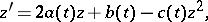
Equation (2) is closely related to the system of differential equations
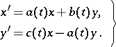 | (3) |
If  is the solution of the system (3) when
  and
and  does not vanish on
  , then
 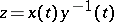 is the solution of (2); if
  is the solution of (2), yet
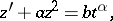
  is the solution of the equation
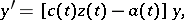 |
then the pair 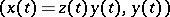 is the solution of (3). In particular, solutions of (2) when
  are related to solutions of the equation
 |
by  if
if  does not vanish on
  . Because of this relation, the equation (2) is often drawn upon for the study of oscillation, non-oscillation (cf. Oscillating differential equation), reducibility (cf. Reducible linear system), and many other questions concerning the qualitative behaviour of linear equations and second-order systems (see [3], [4]).
The equation
 | (4) |
where  is an unknown
  -matrix-function, and the matrix-functions
  ,
,  ,
,  , and
, and  have dimensions
  ,
,  ,
,  , and
, and  , respectively, is called a matrix Riccati equation. The solution
  of the matrix Riccati equation (4) is related to the solutions
  of the linear matrix system
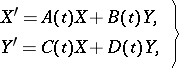 | (5) |
by  .
.
The matrix Riccati equation plays an important part in the theory of linear Hamiltonian systems (cf. Hamiltonian system, linear), the calculus of variations, problems of optimal control, filtration, stabilization of controllable linear systems, etc. (see Control system, and [6], [7]). For example, the optimum control  in the problem of minimization of the functional
 |
on solutions of the system
 |
(the  -matrices
  and
and  are symmetric and non-negative definite, and the
  -matrix
  is positive definite when
  ), is given by the equation
 |
where  is the solution of the matrix Riccati equation
 | (6) |
with the boundary condition  (see [5], [8]).
In problems of control on an infinite time interval, the important questions concern the existence for the matrix Riccati equation of a non-negative definite solution bounded on  , of a periodic or almost-periodic solution (in the case of periodic or almost-periodic coefficients of the equation) and the means of an approximate construction of such solutions.
In variational problems with discrete time and problems of discrete optimization the following recurrent matrix Riccati equation serves as an analogue to equation (4):
 |
Equation (4) can naturally be put into correspondence with a dynamical system on a Grassmann manifold  (see [9]) so that the theory of dynamical systems can be applied to (4). For example, if the matrices
  ,
,  ,
,  , and
, and  in (4) are periodic with period
  and if
  , where
  are the multipliers (see Floquet–Lyapunov theorem) of the system (5), then the corresponding dynamical system is generated by a Morse–Smale diffeomorphism (see Morse–Smale system), and is thus structurally stable.
References
| [1] | J. Riccati, "Opere" , Treviso (1758) |
| [2] | E. Kamke, "Differentialgleichungen: Lösungen und Lösungsmethoden" , 1. Gewöhnliche Differentialgleichungen , Chelsea, reprint (1971) |
| [3] | N.P. Erugin, "A reader for a general course in differential equations" , Minsk (1979) (In Russian) |
| [4] | N.P. Erugin, "Linear systems of ordinary differential equations with periodic and quasi-periodic coefficients" , Acad. Press (1966) (Translated from Russian) |
| [5] | W.T. Reid, "Riccati differential equations" , Acad. Press (1972) |
| [6] | R.E. Kalman, P.L. Falb, M.A. Arbib, "Topics in mathematical systems theory" , McGraw-Hill (1969) |
| [7] | J.-L. Lions, "Optimal control of systems governed by partial differential equations" , Springer (1971) (Translated from French) |
| [8] | M.K. Zakhar-Itkin, "The matrix Riccati differential equation and the semi-group of linear fractional transformations" Russian Math. Surveys , 28 : 3 (1973) pp. 89–131 Uspekhi Mat. Nauk , 28 : 3 (1973) pp. 83–120 |
| [9] | C.R. Schneider, "Global aspects of the matrix Riccati equation" Math Syst. Theory , 7 : 3 (1973) pp. 281–286 |
Comments
The matrix equation  , much related to the existence of equilibria of (4), where
  ,
,  ,
,  ,
,  are given constant matrices, is known as the algebraic Riccati equation.
Riccati equation. Encyclopedia of Mathematics. URL: http://encyclopediaofmath.org/index.php?title=Riccati_equation&oldid=48535