Difference between revisions of "Retarded potentials, method of"
Ulf Rehmann (talk | contribs) m (tex encoded by computer) |
Ulf Rehmann (talk | contribs) m (Undo revision 48532 by Ulf Rehmann (talk)) Tag: Undo |
||
| Line 1: | Line 1: | ||
| − | |||
| − | |||
| − | |||
| − | |||
| − | |||
| − | |||
| − | |||
| − | |||
| − | |||
| − | |||
| − | |||
| − | |||
''Duhamel principle'' | ''Duhamel principle'' | ||
| Line 17: | Line 5: | ||
Consider the equation | Consider the equation | ||
| − | + | <table class="eq" style="width:100%;"> <tr><td valign="top" style="width:94%;text-align:center;"><img align="absmiddle" border="0" src="https://www.encyclopediaofmath.org/legacyimages/r/r081/r081670/r0816701.png" /></td> <td valign="top" style="width:5%;text-align:right;">(1)</td></tr></table> | |
| − | |||
| − | |||
| − | |||
| − | |||
| − | |||
| − | where | + | where <img align="absmiddle" border="0" src="https://www.encyclopediaofmath.org/legacyimages/r/r081/r081670/r0816702.png" /> is an arbitrary linear differential operator involving no derivatives with respect to <img align="absmiddle" border="0" src="https://www.encyclopediaofmath.org/legacyimages/r/r081/r081670/r0816703.png" /> of order higher than <img align="absmiddle" border="0" src="https://www.encyclopediaofmath.org/legacyimages/r/r081/r081670/r0816704.png" />. A particular solution <img align="absmiddle" border="0" src="https://www.encyclopediaofmath.org/legacyimages/r/r081/r081670/r0816705.png" /> of equation (1) (<img align="absmiddle" border="0" src="https://www.encyclopediaofmath.org/legacyimages/r/r081/r081670/r0816706.png" />) is looked for as a [[Duhamel integral|Duhamel integral]]: |
| − | is an arbitrary linear differential operator involving no derivatives with respect to | ||
| − | of order higher than | ||
| − | A particular solution | ||
| − | of equation (1) ( | ||
| − | is looked for as a [[Duhamel integral|Duhamel integral]]: | ||
| − | + | <table class="eq" style="width:100%;"> <tr><td valign="top" style="width:94%;text-align:center;"><img align="absmiddle" border="0" src="https://www.encyclopediaofmath.org/legacyimages/r/r081/r081670/r0816707.png" /></td> <td valign="top" style="width:5%;text-align:right;">(2)</td></tr></table> | |
| − | |||
| − | |||
| − | where | + | where <img align="absmiddle" border="0" src="https://www.encyclopediaofmath.org/legacyimages/r/r081/r081670/r0816708.png" /> is a (regular or generalized) solution of the homogeneous equation |
| − | is a (regular or generalized) solution of the homogeneous equation | ||
| − | + | <table class="eq" style="width:100%;"> <tr><td valign="top" style="width:94%;text-align:center;"><img align="absmiddle" border="0" src="https://www.encyclopediaofmath.org/legacyimages/r/r081/r081670/r0816709.png" /></td> </tr></table> | |
| − | |||
| − | |||
| − | |||
| − | |||
If | If | ||
| − | + | <table class="eq" style="width:100%;"> <tr><td valign="top" style="width:94%;text-align:center;"><img align="absmiddle" border="0" src="https://www.encyclopediaofmath.org/legacyimages/r/r081/r081670/r08167010.png" /></td> </tr></table> | |
| − | |||
| − | |||
| − | |||
| − | |||
| − | then the function (2) obtained by superposition of the impulses | + | then the function (2) obtained by superposition of the impulses <img align="absmiddle" border="0" src="https://www.encyclopediaofmath.org/legacyimages/r/r081/r081670/r08167011.png" /> is a solution to the Cauchy problem |
| − | is a solution to the Cauchy problem | ||
| − | + | <table class="eq" style="width:100%;"> <tr><td valign="top" style="width:94%;text-align:center;"><img align="absmiddle" border="0" src="https://www.encyclopediaofmath.org/legacyimages/r/r081/r081670/r08167012.png" /></td> <td valign="top" style="width:5%;text-align:right;">(3)</td></tr></table> | |
| − | |||
| − | |||
| − | |||
| − | |||
| − | |||
for the inhomogeneous equation (1). | for the inhomogeneous equation (1). | ||
| − | In the case of a system of ordinary differential equations, the method of retarded potentials is known as the method of variation of constants or the method of impulses. For ordinary linear differential equations of order | + | In the case of a system of ordinary differential equations, the method of retarded potentials is known as the method of variation of constants or the method of impulses. For ordinary linear differential equations of order <img align="absmiddle" border="0" src="https://www.encyclopediaofmath.org/legacyimages/r/r081/r081670/r08167013.png" />, |
| − | + | <table class="eq" style="width:100%;"> <tr><td valign="top" style="width:94%;text-align:center;"><img align="absmiddle" border="0" src="https://www.encyclopediaofmath.org/legacyimages/r/r081/r081670/r08167014.png" /></td> <td valign="top" style="width:5%;text-align:right;">(4)</td></tr></table> | |
| − | |||
| − | |||
| − | |||
| − | |||
| − | |||
| − | |||
| − | the method proceeds as follows: if | + | the method proceeds as follows: if <img align="absmiddle" border="0" src="https://www.encyclopediaofmath.org/legacyimages/r/r081/r081670/r08167015.png" /> is any [[Fundamental system of solutions|fundamental system of solutions]] to the equation <img align="absmiddle" border="0" src="https://www.encyclopediaofmath.org/legacyimages/r/r081/r081670/r08167016.png" />, then a solution <img align="absmiddle" border="0" src="https://www.encyclopediaofmath.org/legacyimages/r/r081/r081670/r08167017.png" /> to the inhomogeneous equation (4) is sought for in the form |
| − | is any [[Fundamental system of solutions|fundamental system of solutions]] to the equation | ||
| − | then a solution | ||
| − | to the inhomogeneous equation (4) is sought for in the form | ||
| − | + | <table class="eq" style="width:100%;"> <tr><td valign="top" style="width:94%;text-align:center;"><img align="absmiddle" border="0" src="https://www.encyclopediaofmath.org/legacyimages/r/r081/r081670/r08167018.png" /></td> </tr></table> | |
| − | |||
| − | |||
| − | The functions | + | The functions <img align="absmiddle" border="0" src="https://www.encyclopediaofmath.org/legacyimages/r/r081/r081670/r08167019.png" />, <img align="absmiddle" border="0" src="https://www.encyclopediaofmath.org/legacyimages/r/r081/r081670/r08167020.png" />, are uniquely defined as the set of solutions to the system of algebraic equations |
| − | |||
| − | are uniquely defined as the set of solutions to the system of algebraic equations | ||
| − | + | <table class="eq" style="width:100%;"> <tr><td valign="top" style="width:94%;text-align:center;"><img align="absmiddle" border="0" src="https://www.encyclopediaofmath.org/legacyimages/r/r081/r081670/r08167021.png" /></td> </tr></table> | |
| − | |||
| − | |||
| − | |||
| − | |||
| − | |||
| − | + | <table class="eq" style="width:100%;"> <tr><td valign="top" style="width:94%;text-align:center;"><img align="absmiddle" border="0" src="https://www.encyclopediaofmath.org/legacyimages/r/r081/r081670/r08167022.png" /></td> </tr></table> | |
| − | |||
| − | |||
| − | |||
| − | |||
| − | |||
with non-vanishing [[Wronskian|Wronskian]]. | with non-vanishing [[Wronskian|Wronskian]]. | ||
| − | If | + | If <img align="absmiddle" border="0" src="https://www.encyclopediaofmath.org/legacyimages/r/r081/r081670/r08167023.png" /> for <img align="absmiddle" border="0" src="https://www.encyclopediaofmath.org/legacyimages/r/r081/r081670/r08167024.png" />, the solution <img align="absmiddle" border="0" src="https://www.encyclopediaofmath.org/legacyimages/r/r081/r081670/r08167025.png" /> of the homogeneous Cauchy problem (3) for equation (4) is usually called a normal reaction to the external load <img align="absmiddle" border="0" src="https://www.encyclopediaofmath.org/legacyimages/r/r081/r081670/r08167026.png" />. The function <img align="absmiddle" border="0" src="https://www.encyclopediaofmath.org/legacyimages/r/r081/r081670/r08167027.png" /> can be expressed as a convolution or Duhamel integral: |
| − | for | ||
| − | the solution | ||
| − | of the homogeneous Cauchy problem (3) for equation (4) is usually called a normal reaction to the external load | ||
| − | The function | ||
| − | can be expressed as a convolution or Duhamel integral: | ||
| − | + | <table class="eq" style="width:100%;"> <tr><td valign="top" style="width:94%;text-align:center;"><img align="absmiddle" border="0" src="https://www.encyclopediaofmath.org/legacyimages/r/r081/r081670/r08167028.png" /></td> </tr></table> | |
| − | |||
| − | |||
| − | |||
| − | where | + | where <img align="absmiddle" border="0" src="https://www.encyclopediaofmath.org/legacyimages/r/r081/r081670/r08167029.png" /> for <img align="absmiddle" border="0" src="https://www.encyclopediaofmath.org/legacyimages/r/r081/r081670/r08167030.png" /> and |
| − | for | ||
| − | and | ||
| − | + | <table class="eq" style="width:100%;"> <tr><td valign="top" style="width:94%;text-align:center;"><img align="absmiddle" border="0" src="https://www.encyclopediaofmath.org/legacyimages/r/r081/r081670/r08167031.png" /></td> </tr></table> | |
| − | |||
| − | |||
| − | |||
| − | |||
| − | Let | + | Let <img align="absmiddle" border="0" src="https://www.encyclopediaofmath.org/legacyimages/r/r081/r081670/r08167032.png" />, <img align="absmiddle" border="0" src="https://www.encyclopediaofmath.org/legacyimages/r/r081/r081670/r08167033.png" />, be a function with continuous partial derivatives of order up to <img align="absmiddle" border="0" src="https://www.encyclopediaofmath.org/legacyimages/r/r081/r081670/r08167034.png" /> (if <img align="absmiddle" border="0" src="https://www.encyclopediaofmath.org/legacyimages/r/r081/r081670/r08167035.png" /> is odd) or <img align="absmiddle" border="0" src="https://www.encyclopediaofmath.org/legacyimages/r/r081/r081670/r08167036.png" /> (if <img align="absmiddle" border="0" src="https://www.encyclopediaofmath.org/legacyimages/r/r081/r081670/r08167037.png" /> is even), and let <img align="absmiddle" border="0" src="https://www.encyclopediaofmath.org/legacyimages/r/r081/r081670/r08167038.png" /> be the mean value of <img align="absmiddle" border="0" src="https://www.encyclopediaofmath.org/legacyimages/r/r081/r081670/r08167039.png" /> on the sphere <img align="absmiddle" border="0" src="https://www.encyclopediaofmath.org/legacyimages/r/r081/r081670/r08167040.png" /> with centre <img align="absmiddle" border="0" src="https://www.encyclopediaofmath.org/legacyimages/r/r081/r081670/r08167041.png" /> and radius <img align="absmiddle" border="0" src="https://www.encyclopediaofmath.org/legacyimages/r/r081/r081670/r08167042.png" />. The function |
| − | |||
| − | be a function with continuous partial derivatives of order up to | ||
| − | if | ||
| − | is odd) or | ||
| − | if | ||
| − | is even), and let | ||
| − | be the mean value of | ||
| − | on the sphere | ||
| − | with centre | ||
| − | and radius | ||
| − | The function | ||
| − | + | <table class="eq" style="width:100%;"> <tr><td valign="top" style="width:94%;text-align:center;"><img align="absmiddle" border="0" src="https://www.encyclopediaofmath.org/legacyimages/r/r081/r081670/r08167043.png" /></td> </tr></table> | |
| − | |||
| − | |||
| − | + | <table class="eq" style="width:100%;"> <tr><td valign="top" style="width:94%;text-align:center;"><img align="absmiddle" border="0" src="https://www.encyclopediaofmath.org/legacyimages/r/r081/r081670/r08167044.png" /></td> </tr></table> | |
| − | = | ||
| − | + | which depends on the non-negative parameter <img align="absmiddle" border="0" src="https://www.encyclopediaofmath.org/legacyimages/r/r081/r081670/r08167045.png" />, is a solution to the [[Wave equation|wave equation]] | |
| − | |||
| − | |||
| − | |||
| − | |||
| − | + | <table class="eq" style="width:100%;"> <tr><td valign="top" style="width:94%;text-align:center;"><img align="absmiddle" border="0" src="https://www.encyclopediaofmath.org/legacyimages/r/r081/r081670/r08167046.png" /></td> </tr></table> | |
| − | |||
| − | |||
| − | |||
| − | |||
| − | |||
satisfying the initial conditions | satisfying the initial conditions | ||
| − | + | <table class="eq" style="width:100%;"> <tr><td valign="top" style="width:94%;text-align:center;"><img align="absmiddle" border="0" src="https://www.encyclopediaofmath.org/legacyimages/r/r081/r081670/r08167047.png" /></td> </tr></table> | |
| − | |||
| − | |||
The Duhamel integral | The Duhamel integral | ||
| − | + | <table class="eq" style="width:100%;"> <tr><td valign="top" style="width:94%;text-align:center;"><img align="absmiddle" border="0" src="https://www.encyclopediaofmath.org/legacyimages/r/r081/r081670/r08167048.png" /></td> <td valign="top" style="width:5%;text-align:right;">(5)</td></tr></table> | |
| − | |||
| − | |||
| − | is a solution to the homogeneous Cauchy problem | + | is a solution to the homogeneous Cauchy problem <img align="absmiddle" border="0" src="https://www.encyclopediaofmath.org/legacyimages/r/r081/r081670/r08167049.png" />, <img align="absmiddle" border="0" src="https://www.encyclopediaofmath.org/legacyimages/r/r081/r081670/r08167050.png" /> for the equation <img align="absmiddle" border="0" src="https://www.encyclopediaofmath.org/legacyimages/r/r081/r081670/r08167051.png" />. If <img align="absmiddle" border="0" src="https://www.encyclopediaofmath.org/legacyimages/r/r081/r081670/r08167052.png" /> or <img align="absmiddle" border="0" src="https://www.encyclopediaofmath.org/legacyimages/r/r081/r081670/r08167053.png" />, (5) implies |
| − | |||
| − | for the equation | ||
| − | If | ||
| − | or | ||
| − | (5) implies | ||
| − | + | <table class="eq" style="width:100%;"> <tr><td valign="top" style="width:94%;text-align:center;"><img align="absmiddle" border="0" src="https://www.encyclopediaofmath.org/legacyimages/r/r081/r081670/r08167054.png" /></td> </tr></table> | |
| − | |||
| − | |||
| − | |||
| − | |||
| − | |||
| − | |||
| − | |||
| − | |||
or | or | ||
| − | + | <table class="eq" style="width:100%;"> <tr><td valign="top" style="width:94%;text-align:center;"><img align="absmiddle" border="0" src="https://www.encyclopediaofmath.org/legacyimages/r/r081/r081670/r08167055.png" /></td> <td valign="top" style="width:5%;text-align:right;">(6)</td></tr></table> | |
| − | |||
| − | |||
| − | |||
| − | |||
| − | |||
| − | |||
| − | where | + | where <img align="absmiddle" border="0" src="https://www.encyclopediaofmath.org/legacyimages/r/r081/r081670/r08167056.png" />. |
| − | On the other hand, if | + | On the other hand, if <img align="absmiddle" border="0" src="https://www.encyclopediaofmath.org/legacyimages/r/r081/r081670/r08167057.png" />, then |
| − | then | ||
| − | + | <table class="eq" style="width:100%;"> <tr><td valign="top" style="width:94%;text-align:center;"><img align="absmiddle" border="0" src="https://www.encyclopediaofmath.org/legacyimages/r/r081/r081670/r08167058.png" /></td> </tr></table> | |
| − | |||
| − | |||
| − | |||
| − | |||
| − | The integral in (6) is known as a retarded potential with density | + | The integral in (6) is known as a retarded potential with density <img align="absmiddle" border="0" src="https://www.encyclopediaofmath.org/legacyimages/r/r081/r081670/r08167059.png" />. |
The method of retarded potentials (method of variation of parameters) is particularly simple and useful when applied to first-order linear systems of differential equations of the type | The method of retarded potentials (method of variation of parameters) is particularly simple and useful when applied to first-order linear systems of differential equations of the type | ||
| − | + | <table class="eq" style="width:100%;"> <tr><td valign="top" style="width:94%;text-align:center;"><img align="absmiddle" border="0" src="https://www.encyclopediaofmath.org/legacyimages/r/r081/r081670/r08167060.png" /></td> <td valign="top" style="width:5%;text-align:right;">(7)</td></tr></table> | |
| − | |||
| − | |||
| − | |||
| − | where | + | where <img align="absmiddle" border="0" src="https://www.encyclopediaofmath.org/legacyimages/r/r081/r081670/r08167061.png" /> is a <img align="absmiddle" border="0" src="https://www.encyclopediaofmath.org/legacyimages/r/r081/r081670/r08167062.png" />-dimensional vector, <img align="absmiddle" border="0" src="https://www.encyclopediaofmath.org/legacyimages/r/r081/r081670/r08167063.png" /> and <img align="absmiddle" border="0" src="https://www.encyclopediaofmath.org/legacyimages/r/r081/r081670/r08167064.png" /> are given <img align="absmiddle" border="0" src="https://www.encyclopediaofmath.org/legacyimages/r/r081/r081670/r08167065.png" />-matrices and <img align="absmiddle" border="0" src="https://www.encyclopediaofmath.org/legacyimages/r/r081/r081670/r08167066.png" /> is a given vector. |
| − | is a | ||
| − | dimensional vector, | ||
| − | and | ||
| − | are given | ||
| − | matrices and | ||
| − | is a given vector. | ||
| − | Suppose that the vector | + | Suppose that the vector <img align="absmiddle" border="0" src="https://www.encyclopediaofmath.org/legacyimages/r/r081/r081670/r08167067.png" />, depending on a parameter <img align="absmiddle" border="0" src="https://www.encyclopediaofmath.org/legacyimages/r/r081/r081670/r08167068.png" />, is a solution to the Cauchy problem |
| − | depending on a parameter | ||
| − | is a solution to the Cauchy problem | ||
| − | + | <table class="eq" style="width:100%;"> <tr><td valign="top" style="width:94%;text-align:center;"><img align="absmiddle" border="0" src="https://www.encyclopediaofmath.org/legacyimages/r/r081/r081670/r08167069.png" /></td> </tr></table> | |
| − | |||
| − | |||
| − | for the homogeneous system | + | for the homogeneous system <img align="absmiddle" border="0" src="https://www.encyclopediaofmath.org/legacyimages/r/r081/r081670/r08167070.png" />. Then the vector |
| − | Then the vector | ||
| − | + | <table class="eq" style="width:100%;"> <tr><td valign="top" style="width:94%;text-align:center;"><img align="absmiddle" border="0" src="https://www.encyclopediaofmath.org/legacyimages/r/r081/r081670/r08167071.png" /></td> <td valign="top" style="width:5%;text-align:right;">(8)</td></tr></table> | |
| − | |||
| − | |||
is a solution to the inhomogeneous system (7) with initial condition | is a solution to the inhomogeneous system (7) with initial condition | ||
| − | + | <table class="eq" style="width:100%;"> <tr><td valign="top" style="width:94%;text-align:center;"><img align="absmiddle" border="0" src="https://www.encyclopediaofmath.org/legacyimages/r/r081/r081670/r08167072.png" /></td> <td valign="top" style="width:5%;text-align:right;">(9)</td></tr></table> | |
| − | |||
| − | |||
| − | The function | + | The function <img align="absmiddle" border="0" src="https://www.encyclopediaofmath.org/legacyimages/r/r081/r081670/r08167073.png" /> corresponding to the inhomogeneous [[Heat equation|heat equation]] |
| − | corresponding to the inhomogeneous [[Heat equation|heat equation]] | ||
| − | + | <table class="eq" style="width:100%;"> <tr><td valign="top" style="width:94%;text-align:center;"><img align="absmiddle" border="0" src="https://www.encyclopediaofmath.org/legacyimages/r/r081/r081670/r08167074.png" /></td> <td valign="top" style="width:5%;text-align:right;">(10)</td></tr></table> | |
| − | |||
| − | |||
has the form | has the form | ||
| − | + | <table class="eq" style="width:100%;"> <tr><td valign="top" style="width:94%;text-align:center;"><img align="absmiddle" border="0" src="https://www.encyclopediaofmath.org/legacyimages/r/r081/r081670/r08167075.png" /></td> <td valign="top" style="width:5%;text-align:right;">(11)</td></tr></table> | |
| − | |||
| − | |||
| − | |||
| − | |||
| − | |||
| − | |||
| − | where | + | where <img align="absmiddle" border="0" src="https://www.encyclopediaofmath.org/legacyimages/r/r081/r081670/r08167076.png" /> is the Euclidean space. The solution <img align="absmiddle" border="0" src="https://www.encyclopediaofmath.org/legacyimages/r/r081/r081670/r08167077.png" /> of equation (10) with initial condition (9) is given by a Duhamel integral (3), with the function (11) as integrand. |
| − | is the Euclidean space. The solution | ||
| − | of equation (10) with initial condition (9) is given by a Duhamel integral (3), with the function (11) as integrand. | ||
The method of retarded potentials is also used to investigate mixed problems for partial differential equations of parabolic and hyperbolic types; it enables one to reduce the general problem to problems involving special initial and boundary functions. | The method of retarded potentials is also used to investigate mixed problems for partial differential equations of parabolic and hyperbolic types; it enables one to reduce the general problem to problems involving special initial and boundary functions. | ||
| − | For example, in the domain | + | For example, in the domain <img align="absmiddle" border="0" src="https://www.encyclopediaofmath.org/legacyimages/r/r081/r081670/r08167078.png" />, consider the partial differential equation |
| − | consider the partial differential equation | ||
| − | + | <table class="eq" style="width:100%;"> <tr><td valign="top" style="width:94%;text-align:center;"><img align="absmiddle" border="0" src="https://www.encyclopediaofmath.org/legacyimages/r/r081/r081670/r08167079.png" /></td> <td valign="top" style="width:5%;text-align:right;">(12)</td></tr></table> | |
| − | |||
| − | |||
| − | where | + | where <img align="absmiddle" border="0" src="https://www.encyclopediaofmath.org/legacyimages/r/r081/r081670/r08167080.png" />, <img align="absmiddle" border="0" src="https://www.encyclopediaofmath.org/legacyimages/r/r081/r081670/r08167081.png" />, |
| − | |||
| − | + | <table class="eq" style="width:100%;"> <tr><td valign="top" style="width:94%;text-align:center;"><img align="absmiddle" border="0" src="https://www.encyclopediaofmath.org/legacyimages/r/r081/r081670/r08167082.png" /></td> </tr></table> | |
| − | |||
| − | + | <table class="eq" style="width:100%;"> <tr><td valign="top" style="width:94%;text-align:center;"><img align="absmiddle" border="0" src="https://www.encyclopediaofmath.org/legacyimages/r/r081/r081670/r08167083.png" /></td> </tr></table> | |
| − | |||
| − | which is hyperbolic if | + | which is hyperbolic if <img align="absmiddle" border="0" src="https://www.encyclopediaofmath.org/legacyimages/r/r081/r081670/r08167084.png" /> and parabolic if <img align="absmiddle" border="0" src="https://www.encyclopediaofmath.org/legacyimages/r/r081/r081670/r08167085.png" />. If <img align="absmiddle" border="0" src="https://www.encyclopediaofmath.org/legacyimages/r/r081/r081670/r08167086.png" /> is a continuous solution, differentiable at <img align="absmiddle" border="0" src="https://www.encyclopediaofmath.org/legacyimages/r/r081/r081670/r08167087.png" />, of the mixed problem |
| − | and parabolic if | ||
| − | |||
| − | is a continuous solution, differentiable at | ||
| − | of the mixed problem | ||
| − | + | <table class="eq" style="width:100%;"> <tr><td valign="top" style="width:94%;text-align:center;"><img align="absmiddle" border="0" src="https://www.encyclopediaofmath.org/legacyimages/r/r081/r081670/r08167088.png" /></td> </tr></table> | |
| − | |||
| − | |||
| − | |||
| − | + | <table class="eq" style="width:100%;"> <tr><td valign="top" style="width:94%;text-align:center;"><img align="absmiddle" border="0" src="https://www.encyclopediaofmath.org/legacyimages/r/r081/r081670/r08167089.png" /></td> </tr></table> | |
| − | |||
| − | |||
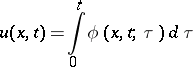
| − | for equation (12) in | + | for equation (12) in <img align="absmiddle" border="0" src="https://www.encyclopediaofmath.org/legacyimages/r/r081/r081670/r08167090.png" />, then, according to the method of retarded potentials, the Duhamel integral |
| − | then, according to the method of retarded potentials, the Duhamel integral | ||
| − | + | <table class="eq" style="width:100%;"> <tr><td valign="top" style="width:94%;text-align:center;"><img align="absmiddle" border="0" src="https://www.encyclopediaofmath.org/legacyimages/r/r081/r081670/r08167091.png" /></td> <td valign="top" style="width:5%;text-align:right;">(13)</td></tr></table> | |
| − | |||
| − | |||
| − | |||
| − | |||
| − | |||
| − | with continuously-differentiable density | + | with continuously-differentiable density <img align="absmiddle" border="0" src="https://www.encyclopediaofmath.org/legacyimages/r/r081/r081670/r08167092.png" />, is a solution to the mixed problem |
| − | is a solution to the mixed problem | ||
| − | + | <table class="eq" style="width:100%;"> <tr><td valign="top" style="width:94%;text-align:center;"><img align="absmiddle" border="0" src="https://www.encyclopediaofmath.org/legacyimages/r/r081/r081670/r08167093.png" /></td> </tr></table> | |
| − | |||
| − | |||
| − | |||
| − | + | <table class="eq" style="width:100%;"> <tr><td valign="top" style="width:94%;text-align:center;"><img align="absmiddle" border="0" src="https://www.encyclopediaofmath.org/legacyimages/r/r081/r081670/r08167094.png" /></td> </tr></table> | |
| − | |||
| − | |||
| − | for equation (12) in | + | for equation (12) in <img align="absmiddle" border="0" src="https://www.encyclopediaofmath.org/legacyimages/r/r081/r081670/r08167095.png" />. |
| − | Essentially, the Duhamel integral (13) is a formula representing a linear operator | + | Essentially, the Duhamel integral (13) is a formula representing a linear operator <img align="absmiddle" border="0" src="https://www.encyclopediaofmath.org/legacyimages/r/r081/r081670/r08167096.png" /> which, given the boundary function <img align="absmiddle" border="0" src="https://www.encyclopediaofmath.org/legacyimages/r/r081/r081670/r08167097.png" />, produces the solution <img align="absmiddle" border="0" src="https://www.encyclopediaofmath.org/legacyimages/r/r081/r081670/r08167098.png" />. Duhamel's integral formula is valid not only for the operator <img align="absmiddle" border="0" src="https://www.encyclopediaofmath.org/legacyimages/r/r081/r081670/r08167099.png" /> of (13), but also for all linear operators <img align="absmiddle" border="0" src="https://www.encyclopediaofmath.org/legacyimages/r/r081/r081670/r081670100.png" /> satisfying the following conditions: |
| − | which, given the boundary function | ||
| − | produces the solution | ||
| − | Duhamel's integral formula is valid not only for the operator | ||
| − | of (13), but also for all linear operators | ||
| − | satisfying the following conditions: | ||
| − | 1) | + | 1) <img align="absmiddle" border="0" src="https://www.encyclopediaofmath.org/legacyimages/r/r081/r081670/r081670101.png" /> is defined for all functions <img align="absmiddle" border="0" src="https://www.encyclopediaofmath.org/legacyimages/r/r081/r081670/r081670102.png" /> vanishing for <img align="absmiddle" border="0" src="https://www.encyclopediaofmath.org/legacyimages/r/r081/r081670/r081670103.png" />, and maps <img align="absmiddle" border="0" src="https://www.encyclopediaofmath.org/legacyimages/r/r081/r081670/r081670104.png" /> to a function <img align="absmiddle" border="0" src="https://www.encyclopediaofmath.org/legacyimages/r/r081/r081670/r081670105.png" /> which also vanishes for <img align="absmiddle" border="0" src="https://www.encyclopediaofmath.org/legacyimages/r/r081/r081670/r081670106.png" />. |
| − | is defined for all functions | ||
| − | vanishing for | ||
| − | and maps | ||
| − | to a function | ||
| − | which also vanishes for | ||
2) | 2) | ||
| − | + | <table class="eq" style="width:100%;"> <tr><td valign="top" style="width:94%;text-align:center;"><img align="absmiddle" border="0" src="https://www.encyclopediaofmath.org/legacyimages/r/r081/r081670/r081670107.png" /></td> </tr></table> | |
| − | |||
| − | |||
| − | |||
| − | |||
| − | |||
| − | |||
| − | |||
| − | + | where <img align="absmiddle" border="0" src="https://www.encyclopediaofmath.org/legacyimages/r/r081/r081670/r081670108.png" /> is some function of <img align="absmiddle" border="0" src="https://www.encyclopediaofmath.org/legacyimages/r/r081/r081670/r081670109.png" /> and the parameter <img align="absmiddle" border="0" src="https://www.encyclopediaofmath.org/legacyimages/r/r081/r081670/r081670110.png" />. | |
| − | and | ||
| − | |||
| − | + | 3) If <img align="absmiddle" border="0" src="https://www.encyclopediaofmath.org/legacyimages/r/r081/r081670/r081670111.png" /> and <img align="absmiddle" border="0" src="https://www.encyclopediaofmath.org/legacyimages/r/r081/r081670/r081670112.png" /> is differentiable, then | |
| − | + | <table class="eq" style="width:100%;"> <tr><td valign="top" style="width:94%;text-align:center;"><img align="absmiddle" border="0" src="https://www.encyclopediaofmath.org/legacyimages/r/r081/r081670/r081670113.png" /></td> </tr></table> | |
| − | |||
| − | |||
| − | |||
| − | |||
| − | 4) If | + | 4) If <img align="absmiddle" border="0" src="https://www.encyclopediaofmath.org/legacyimages/r/r081/r081670/r081670114.png" />, then for all <img align="absmiddle" border="0" src="https://www.encyclopediaofmath.org/legacyimages/r/r081/r081670/r081670115.png" />, |
| − | then for all | ||
| − | + | <table class="eq" style="width:100%;"> <tr><td valign="top" style="width:94%;text-align:center;"><img align="absmiddle" border="0" src="https://www.encyclopediaofmath.org/legacyimages/r/r081/r081670/r081670116.png" /></td> </tr></table> | |
| − | |||
| − | |||
====References==== | ====References==== | ||
<table><TR><TD valign="top">[1]</TD> <TD valign="top"> A.V. Bitsadze, "Equations of mathematical physics" , MIR (1980) (Translated from Russian)</TD></TR><TR><TD valign="top">[2]</TD> <TD valign="top"> L. Bers, F. John, M. Schechter, "Partial differential equations" , Interscience (1964)</TD></TR><TR><TD valign="top">[3]</TD> <TD valign="top"> V.S. Vladimirov, "Equations of mathematical physics" , MIR (1984) (Translated from Russian)</TD></TR><TR><TD valign="top">[4]</TD> <TD valign="top"> R. Courant, D. Hilbert, "Methods of mathematical physics. Partial differential equations" , '''2''' , Interscience (1965) (Translated from German)</TD></TR><TR><TD valign="top">[5]</TD> <TD valign="top"> L.S. Pontryagin, "Ordinary differential equations" , Addison-Wesley (1962) (Translated from Russian)</TD></TR><TR><TD valign="top">[6]</TD> <TD valign="top"> A.N. Tikhonov, A.A. Samarskii, "Equations of mathematical physics" , Pergamon (1963) (Translated from Russian)</TD></TR></table> | <table><TR><TD valign="top">[1]</TD> <TD valign="top"> A.V. Bitsadze, "Equations of mathematical physics" , MIR (1980) (Translated from Russian)</TD></TR><TR><TD valign="top">[2]</TD> <TD valign="top"> L. Bers, F. John, M. Schechter, "Partial differential equations" , Interscience (1964)</TD></TR><TR><TD valign="top">[3]</TD> <TD valign="top"> V.S. Vladimirov, "Equations of mathematical physics" , MIR (1984) (Translated from Russian)</TD></TR><TR><TD valign="top">[4]</TD> <TD valign="top"> R. Courant, D. Hilbert, "Methods of mathematical physics. Partial differential equations" , '''2''' , Interscience (1965) (Translated from German)</TD></TR><TR><TD valign="top">[5]</TD> <TD valign="top"> L.S. Pontryagin, "Ordinary differential equations" , Addison-Wesley (1962) (Translated from Russian)</TD></TR><TR><TD valign="top">[6]</TD> <TD valign="top"> A.N. Tikhonov, A.A. Samarskii, "Equations of mathematical physics" , Pergamon (1963) (Translated from Russian)</TD></TR></table> | ||
Revision as of 14:53, 7 June 2020
Duhamel principle
A method for determining the solution to the homogeneous Cauchy problem for a (system of) inhomogeneous linear partial differential equation(s) in terms of the known solution to the homogeneous equation or system.
Consider the equation
 | (1) |
where  is an arbitrary linear differential operator involving no derivatives with respect to
  of order higher than
  . A particular solution
  of equation (1) (
 ) is looked for as a Duhamel integral:
 | (2) |
where  is a (regular or generalized) solution of the homogeneous equation
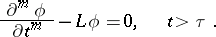 |
If
 |
then the function (2) obtained by superposition of the impulses  is a solution to the Cauchy problem
 | (3) |
for the inhomogeneous equation (1).
In the case of a system of ordinary differential equations, the method of retarded potentials is known as the method of variation of constants or the method of impulses. For ordinary linear differential equations of order  ,
,
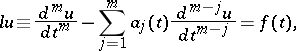 | (4) |
the method proceeds as follows: if  is any fundamental system of solutions to the equation
  , then a solution
  to the inhomogeneous equation (4) is sought for in the form
 |
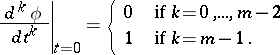
The functions  ,
,  , are uniquely defined as the set of solutions to the system of algebraic equations
 |
 |
with non-vanishing Wronskian.
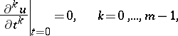
If  for
for  , the solution
  of the homogeneous Cauchy problem (3) for equation (4) is usually called a normal reaction to the external load
  . The function
  can be expressed as a convolution or Duhamel integral:
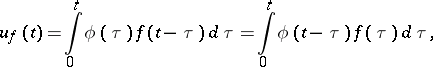 |
where  for
for  and
and
 |
Let  ,
,  , be a function with continuous partial derivatives of order up to
  (if
(if  is odd) or
  (if
(if  is even), and let
  be the mean value of
  on the sphere
  with centre
  and radius
  . The function
 |
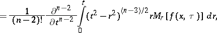 |
which depends on the non-negative parameter  , is a solution to the wave equation
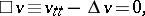 |
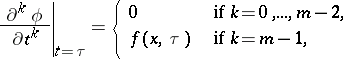
satisfying the initial conditions
 |
The Duhamel integral
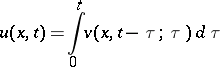 | (5) |
is a solution to the homogeneous Cauchy problem  ,
,  for the equation
  . If
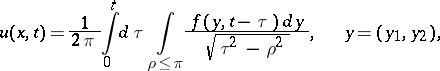
. If  or
or  , (5) implies
 |
or
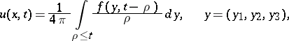 | (6) |
where  .
.
On the other hand, if  , then
 |
The integral in (6) is known as a retarded potential with density  .
.
The method of retarded potentials (method of variation of parameters) is particularly simple and useful when applied to first-order linear systems of differential equations of the type
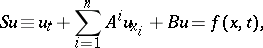 | (7) |
where  is a
is a  -dimensional vector,
  and
and  are given
  -matrices and
  is a given vector.
Suppose that the vector 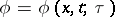 , depending on a parameter
  , is a solution to the Cauchy problem
 |
for the homogeneous system  . Then the vector
 | (8) |
is a solution to the inhomogeneous system (7) with initial condition
 | (9) |
The function  corresponding to the inhomogeneous heat equation
 | (10) |
has the form
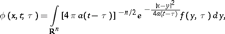 | (11) |
where  is the Euclidean space. The solution
  of equation (10) with initial condition (9) is given by a Duhamel integral (3), with the function (11) as integrand.
The method of retarded potentials is also used to investigate mixed problems for partial differential equations of parabolic and hyperbolic types; it enables one to reduce the general problem to problems involving special initial and boundary functions.
For example, in the domain  , consider the partial differential equation
 | (12) |
where 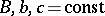 ,
,  ,
,
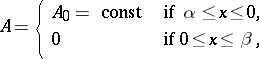 |
 |
which is hyperbolic if  and parabolic if
  . If
. If  is a continuous solution, differentiable at
  , of the mixed problem
 |
 |
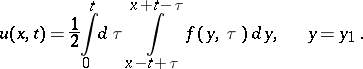
for equation (12) in  , then, according to the method of retarded potentials, the Duhamel integral
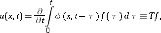 | (13) |
with continuously-differentiable density  , is a solution to the mixed problem
 |
 |
for equation (12) in  .
.
Essentially, the Duhamel integral (13) is a formula representing a linear operator  which, given the boundary function
  , produces the solution
  . Duhamel's integral formula is valid not only for the operator
  of (13), but also for all linear operators
  satisfying the following conditions:
1)  is defined for all functions
  vanishing for
  , and maps
  to a function
  which also vanishes for
  .
.
2)
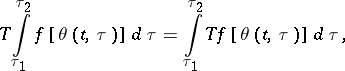 |
where  is some function of
  and the parameter
  .
.
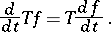
3) If  and
and  is differentiable, then
 |
4) If  , then for all
  ,
,
 |
References
| [1] | A.V. Bitsadze, "Equations of mathematical physics" , MIR (1980) (Translated from Russian) |
| [2] | L. Bers, F. John, M. Schechter, "Partial differential equations" , Interscience (1964) |
| [3] | V.S. Vladimirov, "Equations of mathematical physics" , MIR (1984) (Translated from Russian) |
| [4] | R. Courant, D. Hilbert, "Methods of mathematical physics. Partial differential equations" , 2 , Interscience (1965) (Translated from German) |
| [5] | L.S. Pontryagin, "Ordinary differential equations" , Addison-Wesley (1962) (Translated from Russian) |
| [6] | A.N. Tikhonov, A.A. Samarskii, "Equations of mathematical physics" , Pergamon (1963) (Translated from Russian) |
Retarded potentials, method of. Encyclopedia of Mathematics. URL: http://encyclopediaofmath.org/index.php?title=Retarded_potentials,_method_of&oldid=48532