Difference between revisions of "Pseudo-local tomography"
(Importing text file) |
m (AUTOMATIC EDIT (latexlist): Replaced 68 formulas out of 70 by TEX code with an average confidence of 2.0 and a minimal confidence of 2.0.) |
||
| Line 1: | Line 1: | ||
| − | + | <!--This article has been texified automatically. Since there was no Nroff source code for this article, | |
| + | the semi-automatic procedure described at https://encyclopediaofmath.org/wiki/User:Maximilian_Janisch/latexlist | ||
| + | was used. | ||
| + | If the TeX and formula formatting is correct, please remove this message and the {{TEX|semi-auto}} category. | ||
| − | + | Out of 70 formulas, 68 were replaced by TEX code.--> | |
| + | |||
| + | {{TEX|semi-auto}}{{TEX|partial}} | ||
| + | Let $f ( x )$ be a piecewise smooth, compactly supported function, $x \in \mathbf R ^ { 2 }$. The [[Radon transform|Radon transform]] $\widehat { f } ( \alpha , p ) : = R f$ is defined by the formula $\hat { f } ( \alpha , p ) = \int _ { \operatorname { l_ {\alpha p} } } f ( x ) d s$, where $\text{l} _ { \alpha p} : = \{ x : \alpha \cdot x = p \}$ is a straight line parametrized by a unit vector $\alpha \in S ^ { 1 }$, $S ^ { 1 }$ is the unit circle in $\mathbf{R} ^ { 2 }$ and $p \in \mathbf R _ { + } : = [ 0 , \infty )$. By definition, $\widehat { f } ( - \alpha , - p ) = \widehat { f } ( \alpha , p )$. By local tomographic data one means the values of $\hat { f } ( \alpha , p )$ for $\alpha$ and $p$ satisfying the condition $| \alpha . x _ { 0 } - p | < \rho$, where $x _ { 0 }$ is a given point and $p > 0$ is a small number. Thus, local tomographic data are the line integrals of $f ( x )$ for the lines intersecting the "region of interest" , the disc centred at $x _ { 0 }$ of radius $\rho$ (cf. also [[Local tomography|Local tomography]]; [[Tomography|Tomography]]). | ||
| + | |||
| + | It is not possible, in general, to find $f ( x _ { 0 } )$ from the local tomographic data [[#References|[a2]]]. What practically useful information about $f ( x )$ can one get from these data? Information, very useful practically, is the location of discontinuity curves of $f ( x )$ and the sizes of the jumps of $f ( x )$ across these curves. | ||
Pseudo-local tomography solves the problem of finding the above information from the local tomographic data. | Pseudo-local tomography solves the problem of finding the above information from the local tomographic data. | ||
| Line 7: | Line 15: | ||
This is done by computing the pseudo-local tomography function, introduced in [[#References|[a2]]]: | This is done by computing the pseudo-local tomography function, introduced in [[#References|[a2]]]: | ||
| − | <table class="eq" style="width:100%;"> <tr><td | + | <table class="eq" style="width:100%;"> <tr><td style="width:94%;text-align:center;" valign="top"><img align="absmiddle" border="0" src="https://www.encyclopediaofmath.org/legacyimages/p/p130/p130140/p13014024.png"/></td> <td style="width:5%;text-align:right;" valign="top">(a1)</td></tr></table> |
| − | where | + | where $\widehat { f } _ { p } : = \partial \widehat { f } / \partial p$. The inversion formula reads: |
| − | + | \begin{equation} \tag{a2} f ( x ) = \frac { 1 } { 4 \pi ^ { 2 } } \int _ { S ^ { 1 } } \int _ { - \infty } ^ { \infty } \frac { \hat { f } \rho ( \alpha , p ) } { \alpha . x - p } d p d \alpha, \end{equation} | |
| − | so that (a1) is based on the following idea: Keep a small neighbourhood of the singular point | + | so that (a1) is based on the following idea: Keep a small neighbourhood of the singular point $p = \alpha . x$ in (a1) and neglect the rest of the [[Cauchy integral|Cauchy integral]] in (a1). |
| − | By definition, one needs only the local tomographic data to calculate the pseudo-local tomography function | + | By definition, one needs only the local tomographic data to calculate the pseudo-local tomography function $f _ { \rho } ( x )$. |
| − | The basic result is: | + | The basic result is: $f ( x ) - f _ { \rho } ( x ) \in C ( \mathbf{R} ^ { 2 } )$ is a [[Continuous function|continuous function]] [[#References|[a2]]], [[#References|[a1]]]. |
| − | Therefore, | + | Therefore, $f ( x )$ and $f _ { \rho } ( x )$ have the same discontinuity curves and the same sizes of the jumps across discontinuities. |
| − | It is also proved in [[#References|[a2]]] that if | + | It is also proved in [[#References|[a2]]] that if $f \in C ^ { 2 } ( U )$, where $U \subset \mathbf{R} ^ { 2 }$ is an open set, then the function $f _ { \rho } ^ { C } ( x ) : = f ( x ) - f _ { \rho } ( x )$ has the following properties: |
| − | + | \begin{equation} \tag{a3} | f ^ { C_ \rho } ( x ) - f ( x ) | = O ( \rho )\, \text { as } \rho \rightarrow 0 ,\, x \in U, \end{equation} | |
| − | and the convergence in (a3) is uniform on compact subsets of | + | and the convergence in (a3) is uniform on compact subsets of $U$. If $x _ { 0 } \in S$, where $S$ is a smooth discontinuity curve of $f ( x )$, then |
| − | + | \begin{equation} \tag{a4} \left| f _ { \rho } ^ { C } ( x _ { 0 } ) - \frac { f _+ ( x _ { 0 } ) + f_ - ( x _ { 0 } ) } { 2 } \right| = O ( \rho \operatorname { ln } \rho ) \text { as } \rho \rightarrow 0. \end{equation} | |
| − | Here, | + | Here, $f \pm ( x _ { 0 } )$ are the limiting values of $f ( x )$ as $x \rightarrow x_{0}$ from different sides of $S$ along a path non-tangential to $S$. |
| − | If | + | If $n_0$ is a unit vector normal to $S$ at the point $x _ { 0 }$, then for an arbitrary $\gamma \in \mathbf{R}$, $\gamma \neq 0$, one has |
| − | + | \begin{equation*} \operatorname { lim } _ { \rho \rightarrow 0 } [ f ( x _ { 0 } + \gamma \rho n _ { 0 } ) - f _ { \rho } ^ { C } ( x _ { 0 } + \gamma \rho n _ { 0 } ) ] = D ( x _ { 0 } ) \psi ( \gamma ), \end{equation*} | |
where | where | ||
| − | + | \begin{equation*} D ( x _ { 0 } ) : = \operatorname { lim } _ { t \rightarrow + 0 } [ f ( x _ { 0 } + t n _ { 0 } ) - f ( x - t n _ { 0 } ) ] \end{equation*} | |
and | and | ||
| − | + | \begin{equation*} \psi ( \gamma ) : = \frac { 2 } { \pi ^ { 2 } } \int _ { 0 } ^ { \operatorname { min } ( 1,1 / \gamma ) } \frac { \operatorname { arccos } ( \gamma t ) } { \sqrt { 1 - t ^ { 2 } } } d t , \gamma > 0; \end{equation*} | |
| − | + | \begin{equation*} \psi ( - \gamma ) : = \psi ( \gamma ) , \gamma > 0. \end{equation*} | |
| − | The function | + | The function $\psi ( \gamma ) > 0$, is monotonically decreasing on $\mathbf{R} _ { + }$, $\psi ( + 0 ) = 1 / 2$, |
| − | + | \begin{equation*} \psi ( \gamma ) = \frac { 2 } { \pi ^ { 2 } \gamma } + O \left( \frac { 1 } { \gamma ^ { 3 } } \right) \text { as } \gamma \rightarrow + \infty. \end{equation*} | |
| − | If | + | If $f \in C ^ { k - 1 } ( U _ { \rho } )$, for $k \geq 1$ the $k$th order derivatives of $f ( x )$ exist in $U _ { \rho }$, some of them being discontinuous across $S$, and $S$ is piecewise-smooth in $U _ { \rho }$, then $f _ { \rho } ^ { C } \in C ^ { k } ( U )$. |
| − | Other properties of | + | Other properties of $f _ { \rho }$ can be found in [[#References|[a2]]], which also contains a general method for constructing a family of pseudo-local tomography functions, that is, functions which are computable from local tomographic data and having the same discontinuities and the same sizes of the jumps as $f ( x )$. |
====References==== | ====References==== | ||
| − | <table>< | + | <table><tr><td valign="top">[a1]</td> <td valign="top"> A.G. Ramm, A. Katsevich, "Pseudolocal tomography" ''SIAM J. Appl. Math.'' , '''56''' : 1 (1996) pp. 167–191</td></tr><tr><td valign="top">[a2]</td> <td valign="top"> A.G. Ramm, A. Katsevich, "The Radon transform and local tomography" , CRC (1996)</td></tr></table> |
Revision as of 16:46, 1 July 2020
Let $f ( x )$ be a piecewise smooth, compactly supported function, $x \in \mathbf R ^ { 2 }$. The Radon transform $\widehat { f } ( \alpha , p ) : = R f$ is defined by the formula $\hat { f } ( \alpha , p ) = \int _ { \operatorname { l_ {\alpha p} } } f ( x ) d s$, where $\text{l} _ { \alpha p} : = \{ x : \alpha \cdot x = p \}$ is a straight line parametrized by a unit vector $\alpha \in S ^ { 1 }$, $S ^ { 1 }$ is the unit circle in $\mathbf{R} ^ { 2 }$ and $p \in \mathbf R _ { + } : = [ 0 , \infty )$. By definition, $\widehat { f } ( - \alpha , - p ) = \widehat { f } ( \alpha , p )$. By local tomographic data one means the values of $\hat { f } ( \alpha , p )$ for $\alpha$ and $p$ satisfying the condition $| \alpha . x _ { 0 } - p | < \rho$, where $x _ { 0 }$ is a given point and $p > 0$ is a small number. Thus, local tomographic data are the line integrals of $f ( x )$ for the lines intersecting the "region of interest" , the disc centred at $x _ { 0 }$ of radius $\rho$ (cf. also Local tomography; Tomography).
It is not possible, in general, to find $f ( x _ { 0 } )$ from the local tomographic data [a2]. What practically useful information about $f ( x )$ can one get from these data? Information, very useful practically, is the location of discontinuity curves of $f ( x )$ and the sizes of the jumps of $f ( x )$ across these curves.
Pseudo-local tomography solves the problem of finding the above information from the local tomographic data.
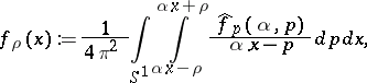
This is done by computing the pseudo-local tomography function, introduced in [a2]:
 | (a1) |
where $\widehat { f } _ { p } : = \partial \widehat { f } / \partial p$. The inversion formula reads:
\begin{equation} \tag{a2} f ( x ) = \frac { 1 } { 4 \pi ^ { 2 } } \int _ { S ^ { 1 } } \int _ { - \infty } ^ { \infty } \frac { \hat { f } \rho ( \alpha , p ) } { \alpha . x - p } d p d \alpha, \end{equation}
so that (a1) is based on the following idea: Keep a small neighbourhood of the singular point $p = \alpha . x$ in (a1) and neglect the rest of the Cauchy integral in (a1).
By definition, one needs only the local tomographic data to calculate the pseudo-local tomography function $f _ { \rho } ( x )$.
The basic result is: $f ( x ) - f _ { \rho } ( x ) \in C ( \mathbf{R} ^ { 2 } )$ is a continuous function [a2], [a1].
Therefore, $f ( x )$ and $f _ { \rho } ( x )$ have the same discontinuity curves and the same sizes of the jumps across discontinuities.
It is also proved in [a2] that if $f \in C ^ { 2 } ( U )$, where $U \subset \mathbf{R} ^ { 2 }$ is an open set, then the function $f _ { \rho } ^ { C } ( x ) : = f ( x ) - f _ { \rho } ( x )$ has the following properties:
\begin{equation} \tag{a3} | f ^ { C_ \rho } ( x ) - f ( x ) | = O ( \rho )\, \text { as } \rho \rightarrow 0 ,\, x \in U, \end{equation}
and the convergence in (a3) is uniform on compact subsets of $U$. If $x _ { 0 } \in S$, where $S$ is a smooth discontinuity curve of $f ( x )$, then
\begin{equation} \tag{a4} \left| f _ { \rho } ^ { C } ( x _ { 0 } ) - \frac { f _+ ( x _ { 0 } ) + f_ - ( x _ { 0 } ) } { 2 } \right| = O ( \rho \operatorname { ln } \rho ) \text { as } \rho \rightarrow 0. \end{equation}
Here, $f \pm ( x _ { 0 } )$ are the limiting values of $f ( x )$ as $x \rightarrow x_{0}$ from different sides of $S$ along a path non-tangential to $S$.
If $n_0$ is a unit vector normal to $S$ at the point $x _ { 0 }$, then for an arbitrary $\gamma \in \mathbf{R}$, $\gamma \neq 0$, one has
\begin{equation*} \operatorname { lim } _ { \rho \rightarrow 0 } [ f ( x _ { 0 } + \gamma \rho n _ { 0 } ) - f _ { \rho } ^ { C } ( x _ { 0 } + \gamma \rho n _ { 0 } ) ] = D ( x _ { 0 } ) \psi ( \gamma ), \end{equation*}
where
\begin{equation*} D ( x _ { 0 } ) : = \operatorname { lim } _ { t \rightarrow + 0 } [ f ( x _ { 0 } + t n _ { 0 } ) - f ( x - t n _ { 0 } ) ] \end{equation*}
and
\begin{equation*} \psi ( \gamma ) : = \frac { 2 } { \pi ^ { 2 } } \int _ { 0 } ^ { \operatorname { min } ( 1,1 / \gamma ) } \frac { \operatorname { arccos } ( \gamma t ) } { \sqrt { 1 - t ^ { 2 } } } d t , \gamma > 0; \end{equation*}
\begin{equation*} \psi ( - \gamma ) : = \psi ( \gamma ) , \gamma > 0. \end{equation*}
The function $\psi ( \gamma ) > 0$, is monotonically decreasing on $\mathbf{R} _ { + }$, $\psi ( + 0 ) = 1 / 2$,
\begin{equation*} \psi ( \gamma ) = \frac { 2 } { \pi ^ { 2 } \gamma } + O \left( \frac { 1 } { \gamma ^ { 3 } } \right) \text { as } \gamma \rightarrow + \infty. \end{equation*}
If $f \in C ^ { k - 1 } ( U _ { \rho } )$, for $k \geq 1$ the $k$th order derivatives of $f ( x )$ exist in $U _ { \rho }$, some of them being discontinuous across $S$, and $S$ is piecewise-smooth in $U _ { \rho }$, then $f _ { \rho } ^ { C } \in C ^ { k } ( U )$.
Other properties of $f _ { \rho }$ can be found in [a2], which also contains a general method for constructing a family of pseudo-local tomography functions, that is, functions which are computable from local tomographic data and having the same discontinuities and the same sizes of the jumps as $f ( x )$.
References
| [a1] | A.G. Ramm, A. Katsevich, "Pseudolocal tomography" SIAM J. Appl. Math. , 56 : 1 (1996) pp. 167–191 |
| [a2] | A.G. Ramm, A. Katsevich, "The Radon transform and local tomography" , CRC (1996) |
Pseudo-local tomography. Encyclopedia of Mathematics. URL: http://encyclopediaofmath.org/index.php?title=Pseudo-local_tomography&oldid=12248