Difference between revisions of "Orthogonal system"
Ulf Rehmann (talk | contribs) m (tex encoded by computer) |
Ulf Rehmann (talk | contribs) m (Undo revision 48080 by Ulf Rehmann (talk)) Tag: Undo |
||
| Line 1: | Line 1: | ||
| − | < | + | An orthogonal system of vectors is a set <img align="absmiddle" border="0" src="https://www.encyclopediaofmath.org/legacyimages/o/o070/o070380/o0703801.png" /> of non-zero vectors of a Euclidean (Hilbert) space with a scalar product <img align="absmiddle" border="0" src="https://www.encyclopediaofmath.org/legacyimages/o/o070/o070380/o0703802.png" /> such that <img align="absmiddle" border="0" src="https://www.encyclopediaofmath.org/legacyimages/o/o070/o070380/o0703803.png" /> when <img align="absmiddle" border="0" src="https://www.encyclopediaofmath.org/legacyimages/o/o070/o070380/o0703804.png" />. If under these conditions the norm of each vector is equal to one, then <img align="absmiddle" border="0" src="https://www.encyclopediaofmath.org/legacyimages/o/o070/o070380/o0703805.png" /> is said to be an [[orthonormal system]]. A complete orthogonal (orthonormal) system of vectors <img align="absmiddle" border="0" src="https://www.encyclopediaofmath.org/legacyimages/o/o070/o070380/o0703806.png" /> is called an orthogonal (orthonormal) basis. |
| − | |||
| − | |||
| − | |||
| − | |||
| − | |||
| − | |||
| − | |||
| − | |||
| − | |||
| − | |||
| − | |||
| − | |||
| − | of non-zero vectors of a Euclidean (Hilbert) space with a scalar product | ||
| − | such that | ||
| − | when | ||
| − | If under these conditions the norm of each vector is equal to one, then | ||
| − | is said to be an [[orthonormal system]]. A complete orthogonal (orthonormal) system of vectors | ||
| − | is called an orthogonal (orthonormal) basis. | ||
''M.I. Voitsekhovskii'' | ''M.I. Voitsekhovskii'' | ||
| − | An orthogonal coordinate system is a coordinate system in which the coordinate lines (or surfaces) intersect at right angles. Orthogonal coordinate systems exist in any Euclidean space, but, generally speaking, do not exist in an arbitrary space. In a two-dimensional smooth affine space, orthogonal systems can always be introduced at least in a sufficiently small neighbourhood of every point. It is sometimes possible to introduce orthogonal coordinate systems in the large. In an orthogonal system, the metric tensor | + | An orthogonal coordinate system is a coordinate system in which the coordinate lines (or surfaces) intersect at right angles. Orthogonal coordinate systems exist in any Euclidean space, but, generally speaking, do not exist in an arbitrary space. In a two-dimensional smooth affine space, orthogonal systems can always be introduced at least in a sufficiently small neighbourhood of every point. It is sometimes possible to introduce orthogonal coordinate systems in the large. In an orthogonal system, the metric tensor <img align="absmiddle" border="0" src="https://www.encyclopediaofmath.org/legacyimages/o/o070/o070380/o0703807.png" /> is diagonal; the diagonal components <img align="absmiddle" border="0" src="https://www.encyclopediaofmath.org/legacyimages/o/o070/o070380/o0703808.png" /> are called Lamé coefficients. The [[Lamé coefficients|Lamé coefficients]] of an orthogonal system in space are expressed by the formulas |
| − | is diagonal; the diagonal components | ||
| − | are called Lamé coefficients. The [[Lamé coefficients|Lamé coefficients]] of an orthogonal system in space are expressed by the formulas | ||
| − | |||
| − | |||
| − | |||
| − | |||
| − | |||
| − | |||
| − | |||
| − | |||
| − | |||
| − | |||
| − | |||
| − | + | <table class="eq" style="width:100%;"> <tr><td valign="top" style="width:94%;text-align:center;"><img align="absmiddle" border="0" src="https://www.encyclopediaofmath.org/legacyimages/o/o070/o070380/o0703809.png" /></td> </tr></table> | |
| − | |||
| − | |||
| − | |||
| − | |||
| − | |||
| − | |||
| − | |||
| − | |||
| − | |||
| − | |||
| − | + | <table class="eq" style="width:100%;"> <tr><td valign="top" style="width:94%;text-align:center;"><img align="absmiddle" border="0" src="https://www.encyclopediaofmath.org/legacyimages/o/o070/o070380/o07038010.png" /></td> </tr></table> | |
| − | |||
| − | |||
| − | + | <table class="eq" style="width:100%;"> <tr><td valign="top" style="width:94%;text-align:center;"><img align="absmiddle" border="0" src="https://www.encyclopediaofmath.org/legacyimages/o/o070/o070380/o07038011.png" /></td> </tr></table> | |
| − | |||
| − | |||
| − | |||
| − | |||
| − | |||
| − | where | + | where <img align="absmiddle" border="0" src="https://www.encyclopediaofmath.org/legacyimages/o/o070/o070380/o07038012.png" />, <img align="absmiddle" border="0" src="https://www.encyclopediaofmath.org/legacyimages/o/o070/o070380/o07038013.png" /> and <img align="absmiddle" border="0" src="https://www.encyclopediaofmath.org/legacyimages/o/o070/o070380/o07038014.png" /> are Cartesian coordinates. The Lamé coefficients are also used to express the line element: |
| − | |||
| − | and | ||
| − | are Cartesian coordinates. The Lamé coefficients are also used to express the line element: | ||
| − | + | <table class="eq" style="width:100%;"> <tr><td valign="top" style="width:94%;text-align:center;"><img align="absmiddle" border="0" src="https://www.encyclopediaofmath.org/legacyimages/o/o070/o070380/o07038015.png" /></td> </tr></table> | |
| − | |||
| − | |||
| − | |||
the element of surface area: | the element of surface area: | ||
| − | + | <table class="eq" style="width:100%;"> <tr><td valign="top" style="width:94%;text-align:center;"><img align="absmiddle" border="0" src="https://www.encyclopediaofmath.org/legacyimages/o/o070/o070380/o07038016.png" /></td> </tr></table> | |
| − | |||
| − | |||
| − | |||
the volume element: | the volume element: | ||
| − | + | <table class="eq" style="width:100%;"> <tr><td valign="top" style="width:94%;text-align:center;"><img align="absmiddle" border="0" src="https://www.encyclopediaofmath.org/legacyimages/o/o070/o070380/o07038017.png" /></td> </tr></table> | |
| − | |||
| − | |||
and the operations of vector analysis: | and the operations of vector analysis: | ||
| − | + | <table class="eq" style="width:100%;"> <tr><td valign="top" style="width:94%;text-align:center;"><img align="absmiddle" border="0" src="https://www.encyclopediaofmath.org/legacyimages/o/o070/o070380/o07038018.png" /></td> </tr></table> | |
| − | |||
| − | |||
| − | |||
| − | |||
| − | |||
| − | |||
| − | |||
| − | |||
| − | |||
| − | |||
| − | |||
| − | + | <table class="eq" style="width:100%;"> <tr><td valign="top" style="width:94%;text-align:center;"><img align="absmiddle" border="0" src="https://www.encyclopediaofmath.org/legacyimages/o/o070/o070380/o07038019.png" /></td> </tr></table> | |
| − | |||
| − | |||
| − | |||
| − | |||
| − | |||
| − | |||
| − | + | <table class="eq" style="width:100%;"> <tr><td valign="top" style="width:94%;text-align:center;"><img align="absmiddle" border="0" src="https://www.encyclopediaofmath.org/legacyimages/o/o070/o070380/o07038020.png" /></td> </tr></table> | |
| − | |||
| − | |||
| − | |||
| − | |||
| − | |||
| − | |||
| − | |||
| − | |||
| − | + | <table class="eq" style="width:100%;"> <tr><td valign="top" style="width:94%;text-align:center;"><img align="absmiddle" border="0" src="https://www.encyclopediaofmath.org/legacyimages/o/o070/o070380/o07038021.png" /></td> </tr></table> | |
| − | |||
| − | + | <table class="eq" style="width:100%;"> <tr><td valign="top" style="width:94%;text-align:center;"><img align="absmiddle" border="0" src="https://www.encyclopediaofmath.org/legacyimages/o/o070/o070380/o07038022.png" /></td> </tr></table> | |
| − | |||
| − | |||
| − | + | <table class="eq" style="width:100%;"> <tr><td valign="top" style="width:94%;text-align:center;"><img align="absmiddle" border="0" src="https://www.encyclopediaofmath.org/legacyimages/o/o070/o070380/o07038023.png" /></td> </tr></table> | |
| − | |||
| − | |||
| − | |||
| − | |||
| − | |||
| − | |||
| − | |||
| − | |||
| − | + | <table class="eq" style="width:100%;"> <tr><td valign="top" style="width:94%;text-align:center;"><img align="absmiddle" border="0" src="https://www.encyclopediaofmath.org/legacyimages/o/o070/o070380/o07038024.png" /></td> </tr></table> | |
| − | |||
| − | |||
| − | |||
| − | |||
| − | |||
| − | |||
| − | |||
| − | |||
| − | + | <table class="eq" style="width:100%;"> <tr><td valign="top" style="width:94%;text-align:center;"><img align="absmiddle" border="0" src="https://www.encyclopediaofmath.org/legacyimages/o/o070/o070380/o07038025.png" /></td> </tr></table> | |
| − | |||
| − | |||
| − | |||
| − | |||
| − | |||
| − | |||
| − | |||
| − | |||
| − | + | <table class="eq" style="width:100%;"> <tr><td valign="top" style="width:94%;text-align:center;"><img align="absmiddle" border="0" src="https://www.encyclopediaofmath.org/legacyimages/o/o070/o070380/o07038026.png" /></td> </tr></table> | |
| − | |||
| − | |||
| − | |||
| − | |||
| − | |||
| − | |||
| − | |||
| − | |||
| − | |||
| − | |||
| − | |||
| − | |||
| − | |||
| − | |||
| − | |||
| − | |||
| − | |||
| − | |||
| − | |||
| − | |||
| − | |||
| − | |||
| − | |||
| − | |||
| − | |||
| − | |||
| − | |||
| − | |||
The most frequently used orthogonal coordinate systems are: on a plane — [[Cartesian coordinates|Cartesian coordinates]]; [[Elliptic coordinates|elliptic coordinates]]; [[Parabolic coordinates|parabolic coordinates]]; and [[Polar coordinates|polar coordinates]]; in space — [[Cylinder coordinates|cylinder coordinates]]; [[Bicylindrical coordinates|bicylindrical coordinates]]; [[Bipolar coordinates|bipolar coordinates]]; [[Paraboloidal coordinates|paraboloidal coordinates]]; and [[Spherical coordinates|spherical coordinates]]. | The most frequently used orthogonal coordinate systems are: on a plane — [[Cartesian coordinates|Cartesian coordinates]]; [[Elliptic coordinates|elliptic coordinates]]; [[Parabolic coordinates|parabolic coordinates]]; and [[Polar coordinates|polar coordinates]]; in space — [[Cylinder coordinates|cylinder coordinates]]; [[Bicylindrical coordinates|bicylindrical coordinates]]; [[Bipolar coordinates|bipolar coordinates]]; [[Paraboloidal coordinates|paraboloidal coordinates]]; and [[Spherical coordinates|spherical coordinates]]. | ||
| Line 186: | Line 47: | ||
''D.D. Sokolov'' | ''D.D. Sokolov'' | ||
| − | An orthogonal system of functions is a finite or countable system of functions | + | An orthogonal system of functions is a finite or countable system of functions <img align="absmiddle" border="0" src="https://www.encyclopediaofmath.org/legacyimages/o/o070/o070380/o07038027.png" /> belonging to a space <img align="absmiddle" border="0" src="https://www.encyclopediaofmath.org/legacyimages/o/o070/o070380/o07038028.png" /> and satisfying the condition |
| − | belonging to a space | ||
| − | and satisfying the condition | ||
| − | |||
| − | |||
| − | |||
| − | |||
| − | |||
| − | |||
| − | |||
| − | |||
| − | |||
| − | |||
| − | |||
| − | |||
| − | + | <table class="eq" style="width:100%;"> <tr><td valign="top" style="width:94%;text-align:center;"><img align="absmiddle" border="0" src="https://www.encyclopediaofmath.org/legacyimages/o/o070/o070380/o07038029.png" /></td> </tr></table> | |
| − | If | + | If <img align="absmiddle" border="0" src="https://www.encyclopediaofmath.org/legacyimages/o/o070/o070380/o07038030.png" /> for all <img align="absmiddle" border="0" src="https://www.encyclopediaofmath.org/legacyimages/o/o070/o070380/o07038031.png" />, then the system is orthonormal. It is supposed that the measure <img align="absmiddle" border="0" src="https://www.encyclopediaofmath.org/legacyimages/o/o070/o070380/o07038032.png" /> defined on the <img align="absmiddle" border="0" src="https://www.encyclopediaofmath.org/legacyimages/o/o070/o070380/o07038033.png" />-algebra <img align="absmiddle" border="0" src="https://www.encyclopediaofmath.org/legacyimages/o/o070/o070380/o07038034.png" /> of subsets of the set <img align="absmiddle" border="0" src="https://www.encyclopediaofmath.org/legacyimages/o/o070/o070380/o07038035.png" /> is countably additive, complete, and has a countable base. This definition encompasses all orthogonal systems studied in analysis. Such systems are obtained for various concrete realizations of the measure space <img align="absmiddle" border="0" src="https://www.encyclopediaofmath.org/legacyimages/o/o070/o070380/o07038036.png" />. |
| − | for all | ||
| − | then the system is orthonormal. It is supposed that the measure | ||
| − | defined on the | ||
| − | algebra | ||
| − | of subsets of the set | ||
| − | is countably additive, complete, and has a countable base. This definition encompasses all orthogonal systems studied in analysis. Such systems are obtained for various concrete realizations of the measure space | ||
| − | The greatest interest is in complete orthonormal systems | + | The greatest interest is in complete orthonormal systems <img align="absmiddle" border="0" src="https://www.encyclopediaofmath.org/legacyimages/o/o070/o070380/o07038037.png" />, which possess the property that for any function <img align="absmiddle" border="0" src="https://www.encyclopediaofmath.org/legacyimages/o/o070/o070380/o07038038.png" /> there is a unique series <img align="absmiddle" border="0" src="https://www.encyclopediaofmath.org/legacyimages/o/o070/o070380/o07038039.png" /> which converges to <img align="absmiddle" border="0" src="https://www.encyclopediaofmath.org/legacyimages/o/o070/o070380/o07038040.png" /> in the metric of the space <img align="absmiddle" border="0" src="https://www.encyclopediaofmath.org/legacyimages/o/o070/o070380/o07038041.png" />. The coefficients <img align="absmiddle" border="0" src="https://www.encyclopediaofmath.org/legacyimages/o/o070/o070380/o07038042.png" /> are defined by the Fourier formula: |
| − | which possess the property that for any function | ||
| − | there is a unique series | ||
| − | which converges to | ||
| − | in the metric of the space | ||
| − | The coefficients | ||
| − | are defined by the Fourier formula: | ||
| − | + | <table class="eq" style="width:100%;"> <tr><td valign="top" style="width:94%;text-align:center;"><img align="absmiddle" border="0" src="https://www.encyclopediaofmath.org/legacyimages/o/o070/o070380/o07038043.png" /></td> </tr></table> | |
| − | |||
| − | |||
| − | These systems exist by virtue of the separability of the space | + | These systems exist by virtue of the separability of the space <img align="absmiddle" border="0" src="https://www.encyclopediaofmath.org/legacyimages/o/o070/o070380/o07038044.png" />. A universal method of constructing complete orthonormal systems is given by the Gram–Schmidt [[Orthogonalization method|orthogonalization method]]. This method can be applied to any complete linearly independent sequence <img align="absmiddle" border="0" src="https://www.encyclopediaofmath.org/legacyimages/o/o070/o070380/o07038045.png" /> of functions in <img align="absmiddle" border="0" src="https://www.encyclopediaofmath.org/legacyimages/o/o070/o070380/o07038046.png" />. |
| − | A universal method of constructing complete orthonormal systems is given by the Gram–Schmidt [[Orthogonalization method|orthogonalization method]]. This method can be applied to any complete linearly independent sequence | ||
| − | of functions in | ||
| − | Important examples of [[Orthogonal series|orthogonal series]] are obtained by considering the space | + | Important examples of [[Orthogonal series|orthogonal series]] are obtained by considering the space <img align="absmiddle" border="0" src="https://www.encyclopediaofmath.org/legacyimages/o/o070/o070380/o07038047.png" /> (in this case, <img align="absmiddle" border="0" src="https://www.encyclopediaofmath.org/legacyimages/o/o070/o070380/o07038048.png" />, <img align="absmiddle" border="0" src="https://www.encyclopediaofmath.org/legacyimages/o/o070/o070380/o07038049.png" /> is the system of Lebesgue-measurable sets and <img align="absmiddle" border="0" src="https://www.encyclopediaofmath.org/legacyimages/o/o070/o070380/o07038050.png" /> is the Lebesgue measure). Many theorems on the convergence or summability of a series <img align="absmiddle" border="0" src="https://www.encyclopediaofmath.org/legacyimages/o/o070/o070380/o07038051.png" /> with respect to a general orthogonal system <img align="absmiddle" border="0" src="https://www.encyclopediaofmath.org/legacyimages/o/o070/o070380/o07038052.png" /> in the space <img align="absmiddle" border="0" src="https://www.encyclopediaofmath.org/legacyimages/o/o070/o070380/o07038053.png" /> are also valid for series with respect to orthonormal systems in the space <img align="absmiddle" border="0" src="https://www.encyclopediaofmath.org/legacyimages/o/o070/o070380/o07038054.png" />. Moreover, in this particular case, interesting concrete orthogonal systems have been constructed which possess some nice properties. These systems include the Haar, Rademacher, Walsh–Paley, and Franklin systems. |
| − | in this case, | ||
| − | |||
| − | is the system of Lebesgue-measurable sets and | ||
| − | is the Lebesgue measure). Many theorems on the convergence or summability of a series | ||
| − | with respect to a general orthogonal system | ||
| − | in the space | ||
| − | are also valid for series with respect to orthonormal systems in the space | ||
| − | Moreover, in this particular case, interesting concrete orthogonal systems have been constructed which possess some nice properties. These systems include the Haar, Rademacher, Walsh–Paley, and Franklin systems. | ||
| − | a) The Haar system | + | a) The Haar system <img align="absmiddle" border="0" src="https://www.encyclopediaofmath.org/legacyimages/o/o070/o070380/o07038055.png" />: <img align="absmiddle" border="0" src="https://www.encyclopediaofmath.org/legacyimages/o/o070/o070380/o07038056.png" />, <img align="absmiddle" border="0" src="https://www.encyclopediaofmath.org/legacyimages/o/o070/o070380/o07038057.png" />, |
| − | |||
| − | |||
| − | + | <table class="eq" style="width:100%;"> <tr><td valign="top" style="width:94%;text-align:center;"><img align="absmiddle" border="0" src="https://www.encyclopediaofmath.org/legacyimages/o/o070/o070380/o07038058.png" /></td> </tr></table> | |
| − | |||
| − | where | + | where <img align="absmiddle" border="0" src="https://www.encyclopediaofmath.org/legacyimages/o/o070/o070380/o07038059.png" />, <img align="absmiddle" border="0" src="https://www.encyclopediaofmath.org/legacyimages/o/o070/o070380/o07038060.png" />, <img align="absmiddle" border="0" src="https://www.encyclopediaofmath.org/legacyimages/o/o070/o070380/o07038061.png" />. Series with respect to the Haar system are typical examples of martingales (cf. [[Martingale|Martingale]]) and thus the general theorems of martingale theory are also correct for them. Moreover, the system <img align="absmiddle" border="0" src="https://www.encyclopediaofmath.org/legacyimages/o/o070/o070380/o07038062.png" /> is a [[Basis|basis]] in <img align="absmiddle" border="0" src="https://www.encyclopediaofmath.org/legacyimages/o/o070/o070380/o07038063.png" />, <img align="absmiddle" border="0" src="https://www.encyclopediaofmath.org/legacyimages/o/o070/o070380/o07038064.png" />, and the Fourier series with respect to the Haar system of any integrable function converges almost-everywhere. |
| − | |||
| − | |||
| − | Series with respect to the Haar system are typical examples of martingales (cf. [[Martingale|Martingale]]) and thus the general theorems of martingale theory are also correct for them. Moreover, the system | ||
| − | is a [[Basis|basis]] in | ||
| − | |||
| − | and the Fourier series with respect to the Haar system of any integrable function converges almost-everywhere. | ||
| − | b) The Rademacher system | + | b) The Rademacher system <img align="absmiddle" border="0" src="https://www.encyclopediaofmath.org/legacyimages/o/o070/o070380/o07038065.png" />: |
| − | + | <table class="eq" style="width:100%;"> <tr><td valign="top" style="width:94%;text-align:center;"><img align="absmiddle" border="0" src="https://www.encyclopediaofmath.org/legacyimages/o/o070/o070380/o07038066.png" /></td> </tr></table> | |
| − | |||
| − | |||
is an important example of a stochastically-independent orthogonal system of functions and is used both in probability theory and in the theory of orthogonal and general series of functions. | is an important example of a stochastically-independent orthogonal system of functions and is used both in probability theory and in the theory of orthogonal and general series of functions. | ||
| − | c) The Walsh–Paley system | + | c) The Walsh–Paley system <img align="absmiddle" border="0" src="https://www.encyclopediaofmath.org/legacyimages/o/o070/o070380/o07038067.png" /> is defined using the Rademacher functions: |
| − | is defined using the Rademacher functions: | ||
| − | + | <table class="eq" style="width:100%;"> <tr><td valign="top" style="width:94%;text-align:center;"><img align="absmiddle" border="0" src="https://www.encyclopediaofmath.org/legacyimages/o/o070/o070380/o07038068.png" /></td> </tr></table> | |
| − | |||
| − | |||
| − | |||
| − | |||
| − | where the numbers | + | where the numbers <img align="absmiddle" border="0" src="https://www.encyclopediaofmath.org/legacyimages/o/o070/o070380/o07038069.png" /> and <img align="absmiddle" border="0" src="https://www.encyclopediaofmath.org/legacyimages/o/o070/o070380/o07038070.png" /> are defined using the binary expansion of the number <img align="absmiddle" border="0" src="https://www.encyclopediaofmath.org/legacyimages/o/o070/o070380/o07038071.png" />: |
| − | and | ||
| − | are defined using the binary expansion of the number | ||
| − | + | <table class="eq" style="width:100%;"> <tr><td valign="top" style="width:94%;text-align:center;"><img align="absmiddle" border="0" src="https://www.encyclopediaofmath.org/legacyimages/o/o070/o070380/o07038072.png" /></td> </tr></table> | |
| − | |||
| − | |||
| − | d) The Franklin system | + | d) The Franklin system <img align="absmiddle" border="0" src="https://www.encyclopediaofmath.org/legacyimages/o/o070/o070380/o07038073.png" /> is obtained by Gram–Schmidt orthogonalization of the sequence of functions |
| − | is obtained by Gram–Schmidt orthogonalization of the sequence of functions | ||
| − | + | <table class="eq" style="width:100%;"> <tr><td valign="top" style="width:94%;text-align:center;"><img align="absmiddle" border="0" src="https://www.encyclopediaofmath.org/legacyimages/o/o070/o070380/o07038074.png" /></td> </tr></table> | |
| − | |||
| − | |||
| − | |||
| − | + | <table class="eq" style="width:100%;"> <tr><td valign="top" style="width:94%;text-align:center;"><img align="absmiddle" border="0" src="https://www.encyclopediaofmath.org/legacyimages/o/o070/o070380/o07038075.png" /></td> </tr></table> | |
| − | |||
| − | |||
| − | It is an example of an orthogonal basis of the space | + | It is an example of an orthogonal basis of the space <img align="absmiddle" border="0" src="https://www.encyclopediaofmath.org/legacyimages/o/o070/o070380/o07038076.png" /> of continuous functions. |
| − | of continuous functions. | ||
In the theory of multiple orthogonal series, function systems of the form | In the theory of multiple orthogonal series, function systems of the form | ||
| − | + | <table class="eq" style="width:100%;"> <tr><td valign="top" style="width:94%;text-align:center;"><img align="absmiddle" border="0" src="https://www.encyclopediaofmath.org/legacyimages/o/o070/o070380/o07038077.png" /></td> </tr></table> | |
| − | |||
| − | |||
| − | + | <table class="eq" style="width:100%;"> <tr><td valign="top" style="width:94%;text-align:center;"><img align="absmiddle" border="0" src="https://www.encyclopediaofmath.org/legacyimages/o/o070/o070380/o07038078.png" /></td> </tr></table> | |
| − | |||
| − | |||
| − | are examined, where | + | are examined, where <img align="absmiddle" border="0" src="https://www.encyclopediaofmath.org/legacyimages/o/o070/o070380/o07038079.png" /> is an orthonormal system in <img align="absmiddle" border="0" src="https://www.encyclopediaofmath.org/legacyimages/o/o070/o070380/o07038080.png" />. These systems are orthonormal on the <img align="absmiddle" border="0" src="https://www.encyclopediaofmath.org/legacyimages/o/o070/o070380/o07038081.png" />-dimensional cube <img align="absmiddle" border="0" src="https://www.encyclopediaofmath.org/legacyimages/o/o070/o070380/o07038082.png" />, and are complete if the system <img align="absmiddle" border="0" src="https://www.encyclopediaofmath.org/legacyimages/o/o070/o070380/o07038083.png" /> is complete. |
| − | is an orthonormal system in | ||
| − | These systems are orthonormal on the | ||
| − | dimensional cube | ||
| − | and are complete if the system | ||
| − | is complete. | ||
====References==== | ====References==== | ||
| Line 316: | Line 103: | ||
====Comments==== | ====Comments==== | ||
| − | A complete system of elements | + | A complete system of elements <img align="absmiddle" border="0" src="https://www.encyclopediaofmath.org/legacyimages/o/o070/o070380/o07038084.png" /> in a Hilbert space, or, more generally, an inner product space <img align="absmiddle" border="0" src="https://www.encyclopediaofmath.org/legacyimages/o/o070/o070380/o07038085.png" />, is a set of elements such that for any <img align="absmiddle" border="0" src="https://www.encyclopediaofmath.org/legacyimages/o/o070/o070380/o07038086.png" />, if <img align="absmiddle" border="0" src="https://www.encyclopediaofmath.org/legacyimages/o/o070/o070380/o07038087.png" /> for all <img align="absmiddle" border="0" src="https://www.encyclopediaofmath.org/legacyimages/o/o070/o070380/o07038088.png" />, then <img align="absmiddle" border="0" src="https://www.encyclopediaofmath.org/legacyimages/o/o070/o070380/o07038089.png" />. |
| − | in a Hilbert space, or, more generally, an inner product space | ||
| − | is a set of elements such that for any | ||
| − | if | ||
| − | for all | ||
| − | then | ||
| − | Cf. also [[Complete system of functions|Complete system of functions]]. The Walsh–Paley system is a complete orthonormal system in | + | Cf. also [[Complete system of functions|Complete system of functions]]. The Walsh–Paley system is a complete orthonormal system in <img align="absmiddle" border="0" src="https://www.encyclopediaofmath.org/legacyimages/o/o070/o070380/o07038090.png" />. |
Revision as of 14:52, 7 June 2020
An orthogonal system of vectors is a set  of non-zero vectors of a Euclidean (Hilbert) space with a scalar product
  such that
  when
when  . If under these conditions the norm of each vector is equal to one, then
  is said to be an orthonormal system. A complete orthogonal (orthonormal) system of vectors
  is called an orthogonal (orthonormal) basis.
M.I. Voitsekhovskii
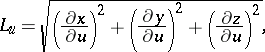
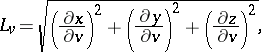
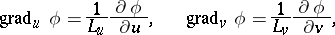
An orthogonal coordinate system is a coordinate system in which the coordinate lines (or surfaces) intersect at right angles. Orthogonal coordinate systems exist in any Euclidean space, but, generally speaking, do not exist in an arbitrary space. In a two-dimensional smooth affine space, orthogonal systems can always be introduced at least in a sufficiently small neighbourhood of every point. It is sometimes possible to introduce orthogonal coordinate systems in the large. In an orthogonal system, the metric tensor  is diagonal; the diagonal components
  are called Lamé coefficients. The Lamé coefficients of an orthogonal system in space are expressed by the formulas
 |
 |
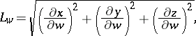 |
where  ,
,  and
and  are Cartesian coordinates. The Lamé coefficients are also used to express the line element:
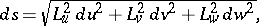 |
the element of surface area:
 |
the volume element:
 |
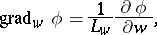
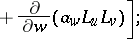
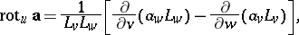
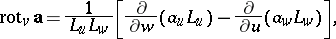
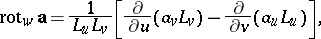
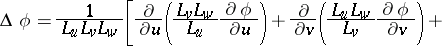
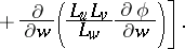
and the operations of vector analysis:
 |
 |
 |
 |
 |
 |
 |
 |
 |
The most frequently used orthogonal coordinate systems are: on a plane — Cartesian coordinates; elliptic coordinates; parabolic coordinates; and polar coordinates; in space — cylinder coordinates; bicylindrical coordinates; bipolar coordinates; paraboloidal coordinates; and spherical coordinates.
D.D. Sokolov
An orthogonal system of functions is a finite or countable system of functions  belonging to a space
  and satisfying the condition
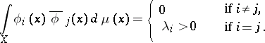 |
If  for all
  , then the system is orthonormal. It is supposed that the measure
  defined on the
  -algebra
  of subsets of the set
  is countably additive, complete, and has a countable base. This definition encompasses all orthogonal systems studied in analysis. Such systems are obtained for various concrete realizations of the measure space
  .
.
The greatest interest is in complete orthonormal systems  , which possess the property that for any function
  there is a unique series
  which converges to
  in the metric of the space
  . The coefficients
  are defined by the Fourier formula:
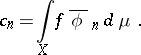 |
These systems exist by virtue of the separability of the space  . A universal method of constructing complete orthonormal systems is given by the Gram–Schmidt orthogonalization method. This method can be applied to any complete linearly independent sequence
  of functions in
  .
.
Important examples of orthogonal series are obtained by considering the space  (in this case,
  ,
,  is the system of Lebesgue-measurable sets and
  is the Lebesgue measure). Many theorems on the convergence or summability of a series
  with respect to a general orthogonal system
  in the space
  are also valid for series with respect to orthonormal systems in the space
  . Moreover, in this particular case, interesting concrete orthogonal systems have been constructed which possess some nice properties. These systems include the Haar, Rademacher, Walsh–Paley, and Franklin systems.
a) The Haar system  :
:  ,
,  ,
,
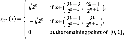 |
where  ,
,  ,
,  . Series with respect to the Haar system are typical examples of martingales (cf. Martingale) and thus the general theorems of martingale theory are also correct for them. Moreover, the system
  is a basis in
  ,
,  , and the Fourier series with respect to the Haar system of any integrable function converges almost-everywhere.
b) The Rademacher system  :
:
 |
is an important example of a stochastically-independent orthogonal system of functions and is used both in probability theory and in the theory of orthogonal and general series of functions.
c) The Walsh–Paley system  is defined using the Rademacher functions:
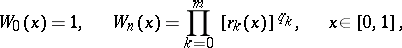 |
where the numbers  and
and  are defined using the binary expansion of the number
  :
:
 |
d) The Franklin system  is obtained by Gram–Schmidt orthogonalization of the sequence of functions
 |
 |
It is an example of an orthogonal basis of the space  of continuous functions.
In the theory of multiple orthogonal series, function systems of the form
 |
 |
are examined, where  is an orthonormal system in
  . These systems are orthonormal on the
  -dimensional cube
  , and are complete if the system
  is complete.
References
| [1] | S. Kaczmarz, H. Steinhaus, "Theorie der Orthogonalreihen" , Chelsea, reprint (1951) |
| [2] | B.I. Golubov, "Series with respect to the Haar system" J. Soviet Math. , 1 : 6 (1973) pp. 704–726 Itogi Nauk. Mat. Anal. 1970 (1971) pp. 109–146 |
| [3] | L.A. Balashov, A.I. Rubenshtein, "Series with respect to the Walsh system and their generalizations" J. Soviet Math. , 1 : 6 (1973) pp. 727–763 Itogi Nauk. Mat. Anal. 1970 (1971) pp. 147–202 |
| [4] | J.L. Doob, "Stochastic processes" , Chapman & Hall (1953) |
| [5] | M. Loève, "Probability theory" , Springer (1977) |
| [6] | A. Zygmund, "Trigonometric series" , 1–2 , Cambridge Univ. Press (1988) |
A.A. Talalyan
Comments
A complete system of elements  in a Hilbert space, or, more generally, an inner product space
  , is a set of elements such that for any
  , if
, if  for all
  , then
  .
.
Cf. also Complete system of functions. The Walsh–Paley system is a complete orthonormal system in  .
.
Orthogonal system. Encyclopedia of Mathematics. URL: http://encyclopediaofmath.org/index.php?title=Orthogonal_system&oldid=48080