Difference between revisions of "Orthogonal polynomials"
Ulf Rehmann (talk | contribs) m (tex encoded by computer) |
Ulf Rehmann (talk | contribs) m (Undo revision 48076 by Ulf Rehmann (talk)) Tag: Undo |
||
| Line 1: | Line 1: | ||
| − | < | + | A system of polynomials <img align="absmiddle" border="0" src="https://www.encyclopediaofmath.org/legacyimages/o/o070/o070340/o0703401.png" /> which satisfy the condition of orthogonality |
| − | |||
| − | |||
| − | |||
| − | |||
| − | |||
| − | |||
| − | |||
| − | + | <table class="eq" style="width:100%;"> <tr><td valign="top" style="width:94%;text-align:center;"><img align="absmiddle" border="0" src="https://www.encyclopediaofmath.org/legacyimages/o/o070/o070340/o0703402.png" /></td> </tr></table> | |
| − | |||
| − | + | whereby the degree of every polynomial <img align="absmiddle" border="0" src="https://www.encyclopediaofmath.org/legacyimages/o/o070/o070340/o0703403.png" /> is equal to its index <img align="absmiddle" border="0" src="https://www.encyclopediaofmath.org/legacyimages/o/o070/o070340/o0703404.png" />, and the weight function (weight) <img align="absmiddle" border="0" src="https://www.encyclopediaofmath.org/legacyimages/o/o070/o070340/o0703405.png" /> on the interval <img align="absmiddle" border="0" src="https://www.encyclopediaofmath.org/legacyimages/o/o070/o070340/o0703406.png" /> or (when <img align="absmiddle" border="0" src="https://www.encyclopediaofmath.org/legacyimages/o/o070/o070340/o0703407.png" /> and <img align="absmiddle" border="0" src="https://www.encyclopediaofmath.org/legacyimages/o/o070/o070340/o0703408.png" /> are finite) on <img align="absmiddle" border="0" src="https://www.encyclopediaofmath.org/legacyimages/o/o070/o070340/o0703409.png" />. Orthogonal polynomials are said to be orthonormalized, and are denoted by <img align="absmiddle" border="0" src="https://www.encyclopediaofmath.org/legacyimages/o/o070/o070340/o07034010.png" />, if every polynomial has positive leading coefficient and if the normalizing condition | |
| − | |||
| − | + | <table class="eq" style="width:100%;"> <tr><td valign="top" style="width:94%;text-align:center;"><img align="absmiddle" border="0" src="https://www.encyclopediaofmath.org/legacyimages/o/o070/o070340/o07034011.png" /></td> </tr></table> | |
| − | |||
| − | |||
| − | |||
| − | + | is fulfilled. If the leading coefficient of each polynomial is equal to 1, then the system of orthogonal polynomials is denoted by <img align="absmiddle" border="0" src="https://www.encyclopediaofmath.org/legacyimages/o/o070/o070340/o07034012.png" />. | |
| − | is equal to | ||
| − | |||
| − | |||
| − | |||
| − | |||
| − | |||
| − | |||
| − | |||
| − | + | The system of orthogonal polynomials <img align="absmiddle" border="0" src="https://www.encyclopediaofmath.org/legacyimages/o/o070/o070340/o07034013.png" /> is uniquely defined if the weight function (differential weight) <img align="absmiddle" border="0" src="https://www.encyclopediaofmath.org/legacyimages/o/o070/o070340/o07034014.png" /> is Lebesgue integrable on <img align="absmiddle" border="0" src="https://www.encyclopediaofmath.org/legacyimages/o/o070/o070340/o07034015.png" />, is not equivalent to zero and, in the case of an unbounded interval <img align="absmiddle" border="0" src="https://www.encyclopediaofmath.org/legacyimages/o/o070/o070340/o07034016.png" />, has finite moments | |
| − | |||
| − | |||
| − | + | <table class="eq" style="width:100%;"> <tr><td valign="top" style="width:94%;text-align:center;"><img align="absmiddle" border="0" src="https://www.encyclopediaofmath.org/legacyimages/o/o070/o070340/o07034017.png" /></td> </tr></table> | |
| − | + | Instead of a differential weight <img align="absmiddle" border="0" src="https://www.encyclopediaofmath.org/legacyimages/o/o070/o070340/o07034018.png" />, an integral weight <img align="absmiddle" border="0" src="https://www.encyclopediaofmath.org/legacyimages/o/o070/o070340/o07034019.png" /> can be examined, where <img align="absmiddle" border="0" src="https://www.encyclopediaofmath.org/legacyimages/o/o070/o070340/o07034020.png" /> is a bounded non-decreasing function with an infinite set of points of growth (in this case, the integral in the condition of orthogonality is understood in the Lebesgue–Stieltjes sense). | |
| − | |||
| − | |||
| − | is | ||
| − | |||
| − | + | For the polynomial <img align="absmiddle" border="0" src="https://www.encyclopediaofmath.org/legacyimages/o/o070/o070340/o07034021.png" /> of degree <img align="absmiddle" border="0" src="https://www.encyclopediaofmath.org/legacyimages/o/o070/o070340/o07034022.png" /> to be part of the system <img align="absmiddle" border="0" src="https://www.encyclopediaofmath.org/legacyimages/o/o070/o070340/o07034023.png" /> with weight <img align="absmiddle" border="0" src="https://www.encyclopediaofmath.org/legacyimages/o/o070/o070340/o07034024.png" />, it is necessary and sufficient that, for any polynomial <img align="absmiddle" border="0" src="https://www.encyclopediaofmath.org/legacyimages/o/o070/o070340/o07034025.png" /> of degree <img align="absmiddle" border="0" src="https://www.encyclopediaofmath.org/legacyimages/o/o070/o070340/o07034026.png" />, the condition | |
| − | |||
| − | |||
| − | + | <table class="eq" style="width:100%;"> <tr><td valign="top" style="width:94%;text-align:center;"><img align="absmiddle" border="0" src="https://www.encyclopediaofmath.org/legacyimages/o/o070/o070340/o07034027.png" /></td> </tr></table> | |
| − | |||
| − | |||
| − | |||
| − | + | is fulfilled. If the interval of orthogonality <img align="absmiddle" border="0" src="https://www.encyclopediaofmath.org/legacyimages/o/o070/o070340/o07034028.png" /> is symmetric with respect to the origin and the weight function <img align="absmiddle" border="0" src="https://www.encyclopediaofmath.org/legacyimages/o/o070/o070340/o07034029.png" /> is even, then every polynomial <img align="absmiddle" border="0" src="https://www.encyclopediaofmath.org/legacyimages/o/o070/o070340/o07034030.png" /> contains only those degrees of <img align="absmiddle" border="0" src="https://www.encyclopediaofmath.org/legacyimages/o/o070/o070340/o07034031.png" /> which have the parity of the number <img align="absmiddle" border="0" src="https://www.encyclopediaofmath.org/legacyimages/o/o070/o070340/o07034032.png" />, i.e. one has the identity | |
| − | of | ||
| − | to | ||
| − | |||
| − | |||
| − | of | ||
| − | the | ||
| − | + | <table class="eq" style="width:100%;"> <tr><td valign="top" style="width:94%;text-align:center;"><img align="absmiddle" border="0" src="https://www.encyclopediaofmath.org/legacyimages/o/o070/o070340/o07034033.png" /></td> </tr></table> | |
| − | |||
| − | |||
| − | + | The zeros of orthogonal polynomials in the case of the interval <img align="absmiddle" border="0" src="https://www.encyclopediaofmath.org/legacyimages/o/o070/o070340/o07034034.png" /> are all real, different and distributed within <img align="absmiddle" border="0" src="https://www.encyclopediaofmath.org/legacyimages/o/o070/o070340/o07034035.png" />, while between two neighbouring zeros of the polynomial <img align="absmiddle" border="0" src="https://www.encyclopediaofmath.org/legacyimages/o/o070/o070340/o07034036.png" /> there is one zero of the polynomial <img align="absmiddle" border="0" src="https://www.encyclopediaofmath.org/legacyimages/o/o070/o070340/o07034037.png" />. Zeros of orthogonal polynomials are often used as interpolation points and in quadrature formulas. | |
| − | |||
| − | |||
| − | |||
| − | |||
| − | |||
| − | |||
| − | |||
| − | |||
| − | |||
| − | |||
| − | The zeros of orthogonal polynomials in the case of the interval | ||
| − | are all real, different and distributed within | ||
| − | while between two neighbouring zeros of the polynomial | ||
| − | there is one zero of the polynomial | ||
| − | Zeros of orthogonal polynomials are often used as interpolation points and in quadrature formulas. | ||
Any three consecutive polynomials of a system of orthogonal polynomials are related by a recurrence formula | Any three consecutive polynomials of a system of orthogonal polynomials are related by a recurrence formula | ||
| − | + | <table class="eq" style="width:100%;"> <tr><td valign="top" style="width:94%;text-align:center;"><img align="absmiddle" border="0" src="https://www.encyclopediaofmath.org/legacyimages/o/o070/o070340/o07034038.png" /></td> </tr></table> | |
| − | |||
| − | |||
| − | |||
| − | |||
where | where | ||
| − | + | <table class="eq" style="width:100%;"> <tr><td valign="top" style="width:94%;text-align:center;"><img align="absmiddle" border="0" src="https://www.encyclopediaofmath.org/legacyimages/o/o070/o070340/o07034039.png" /></td> </tr></table> | |
| − | |||
| − | |||
| − | |||
| − | |||
| − | |||
| − | |||
| − | + | <table class="eq" style="width:100%;"> <tr><td valign="top" style="width:94%;text-align:center;"><img align="absmiddle" border="0" src="https://www.encyclopediaofmath.org/legacyimages/o/o070/o070340/o07034040.png" /></td> </tr></table> | |
| − | |||
| − | |||
| − | + | <table class="eq" style="width:100%;"> <tr><td valign="top" style="width:94%;text-align:center;"><img align="absmiddle" border="0" src="https://www.encyclopediaofmath.org/legacyimages/o/o070/o070340/o07034041.png" /></td> </tr></table> | |
| − | |||
| − | |||
| − | |||
| − | |||
| − | - | + | <table class="eq" style="width:100%;"> <tr><td valign="top" style="width:94%;text-align:center;"><img align="absmiddle" border="0" src="https://www.encyclopediaofmath.org/legacyimages/o/o070/o070340/o07034042.png" /></td> </tr></table> |
| − | |||
| − | |||
| − | |||
| − | + | <table class="eq" style="width:100%;"> <tr><td valign="top" style="width:94%;text-align:center;"><img align="absmiddle" border="0" src="https://www.encyclopediaofmath.org/legacyimages/o/o070/o070340/o07034043.png" /></td> </tr></table> | |
| − | |||
| − | |||
| − | |||
| − | |||
| − | |||
| − | |||
| − | |||
| − | The number | + | The number <img align="absmiddle" border="0" src="https://www.encyclopediaofmath.org/legacyimages/o/o070/o070340/o07034044.png" /> is a normalization factor of the polynomial <img align="absmiddle" border="0" src="https://www.encyclopediaofmath.org/legacyimages/o/o070/o070340/o07034045.png" />, such that the system <img align="absmiddle" border="0" src="https://www.encyclopediaofmath.org/legacyimages/o/o070/o070340/o07034046.png" /> is orthonormalized, i.e. |
| − | is a normalization factor of the polynomial | ||
| − | such that the system | ||
| − | is orthonormalized, i.e. | ||
| − | + | <table class="eq" style="width:100%;"> <tr><td valign="top" style="width:94%;text-align:center;"><img align="absmiddle" border="0" src="https://www.encyclopediaofmath.org/legacyimages/o/o070/o070340/o07034047.png" /></td> </tr></table> | |
| − | |||
| − | |||
For orthogonal polynomials one has the Christoffel–Darboux formula: | For orthogonal polynomials one has the Christoffel–Darboux formula: | ||
| − | + | <table class="eq" style="width:100%;"> <tr><td valign="top" style="width:94%;text-align:center;"><img align="absmiddle" border="0" src="https://www.encyclopediaofmath.org/legacyimages/o/o070/o070340/o07034048.png" /></td> </tr></table> | |
| − | |||
| − | |||
| − | |||
| − | |||
| − | |||
| − | |||
| − | = | ||
| − | + | <table class="eq" style="width:100%;"> <tr><td valign="top" style="width:94%;text-align:center;"><img align="absmiddle" border="0" src="https://www.encyclopediaofmath.org/legacyimages/o/o070/o070340/o07034049.png" /></td> </tr></table> | |
| − | |||
| − | |||
| − | |||
| − | |||
| − | |||
| − | |||
| − | |||
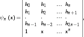
| − | Orthogonal polynomials are represented in terms of the moments | + | Orthogonal polynomials are represented in terms of the moments <img align="absmiddle" border="0" src="https://www.encyclopediaofmath.org/legacyimages/o/o070/o070340/o07034050.png" /> of the weight function <img align="absmiddle" border="0" src="https://www.encyclopediaofmath.org/legacyimages/o/o070/o070340/o07034051.png" /> by the formula |
| − | of the weight function | ||
| − | by the formula | ||
| − | + | <table class="eq" style="width:100%;"> <tr><td valign="top" style="width:94%;text-align:center;"><img align="absmiddle" border="0" src="https://www.encyclopediaofmath.org/legacyimages/o/o070/o070340/o07034052.png" /></td> </tr></table> | |
| − | |||
| − | |||
| − | |||
| − | |||
where | where | ||
| − | + | <table class="eq" style="width:100%;"> <tr><td valign="top" style="width:94%;text-align:center;"><img align="absmiddle" border="0" src="https://www.encyclopediaofmath.org/legacyimages/o/o070/o070340/o07034053.png" /></td> </tr></table> | |
| − | |||
| − | while the determinant | + | while the determinant <img align="absmiddle" border="0" src="https://www.encyclopediaofmath.org/legacyimages/o/o070/o070340/o07034054.png" /> is obtained from <img align="absmiddle" border="0" src="https://www.encyclopediaofmath.org/legacyimages/o/o070/o070340/o07034055.png" /> by cancelling the last row and column and <img align="absmiddle" border="0" src="https://www.encyclopediaofmath.org/legacyimages/o/o070/o070340/o07034056.png" /> is defined in the same way from <img align="absmiddle" border="0" src="https://www.encyclopediaofmath.org/legacyimages/o/o070/o070340/o07034057.png" />. |
| − | is obtained from | ||
| − | by cancelling the last row and column and | ||
| − | is defined in the same way from | ||
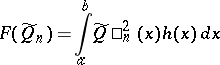
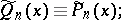
| − | On a set of polynomials | + | On a set of polynomials <img align="absmiddle" border="0" src="https://www.encyclopediaofmath.org/legacyimages/o/o070/o070340/o07034058.png" /> of degree <img align="absmiddle" border="0" src="https://www.encyclopediaofmath.org/legacyimages/o/o070/o070340/o07034059.png" /> with leading coefficient equal to one, the minimum of the functional |
| − | of degree | ||
| − | with leading coefficient equal to one, the minimum of the functional | ||
| − | + | <table class="eq" style="width:100%;"> <tr><td valign="top" style="width:94%;text-align:center;"><img align="absmiddle" border="0" src="https://www.encyclopediaofmath.org/legacyimages/o/o070/o070340/o07034060.png" /></td> </tr></table> | |
| − | |||
| − | |||
is achieved if and only if | is achieved if and only if | ||
| − | + | <table class="eq" style="width:100%;"> <tr><td valign="top" style="width:94%;text-align:center;"><img align="absmiddle" border="0" src="https://www.encyclopediaofmath.org/legacyimages/o/o070/o070340/o07034061.png" /></td> </tr></table> | |
| − | |||
| − | |||
| − | |||
| − | |||
| − | |||
| − | |||
| − | |||
| − | |||
| − | |||
| − | |||
| − | + | moreover, this minimum is equal to <img align="absmiddle" border="0" src="https://www.encyclopediaofmath.org/legacyimages/o/o070/o070340/o07034062.png" />. | |
| − | |||
| − | |||
| − | |||
| − | are orthonormal with weight | + | If the polynomials <img align="absmiddle" border="0" src="https://www.encyclopediaofmath.org/legacyimages/o/o070/o070340/o07034063.png" /> are orthonormal with weight <img align="absmiddle" border="0" src="https://www.encyclopediaofmath.org/legacyimages/o/o070/o070340/o07034064.png" /> on the segment <img align="absmiddle" border="0" src="https://www.encyclopediaofmath.org/legacyimages/o/o070/o070340/o07034065.png" />, then when <img align="absmiddle" border="0" src="https://www.encyclopediaofmath.org/legacyimages/o/o070/o070340/o07034066.png" />, the polynomials |
| − | on the segment | ||
| − | |||
| − | |||
| − | |||
| − | |||
| − | + | <table class="eq" style="width:100%;"> <tr><td valign="top" style="width:94%;text-align:center;"><img align="absmiddle" border="0" src="https://www.encyclopediaofmath.org/legacyimages/o/o070/o070340/o07034067.png" /></td> </tr></table> | |
| − | |||
| − | |||
| − | |||
| − | |||
| − | |||
| − | |||
| − | |||
| − | |||
| − | |||
| − | |||
| − | |||
| − | |||
| − | |||
| − | |||
| − | |||
| − | |||
| − | |||
| − | |||
| − | |||
| − | + | are orthonormal with weight <img align="absmiddle" border="0" src="https://www.encyclopediaofmath.org/legacyimages/o/o070/o070340/o07034068.png" /> on the segment <img align="absmiddle" border="0" src="https://www.encyclopediaofmath.org/legacyimages/o/o070/o070340/o07034069.png" /> which transfers to the segment <img align="absmiddle" border="0" src="https://www.encyclopediaofmath.org/legacyimages/o/o070/o070340/o07034070.png" /> as a result of the linear transformation <img align="absmiddle" border="0" src="https://www.encyclopediaofmath.org/legacyimages/o/o070/o070340/o07034071.png" />. For this reason, when studying the asymptotic properties of orthogonal polynomials, the case of the standard segment <img align="absmiddle" border="0" src="https://www.encyclopediaofmath.org/legacyimages/o/o070/o070340/o07034072.png" /> is considered first, while the results thus obtained cover other cases as well. | |
| − | of the | ||
| − | |||
| − | + | The most important orthogonal polynomials encountered in solving boundary problems of mathematical physics are the so-called [[Classical orthogonal polynomials|classical orthogonal polynomials]]: the [[Laguerre polynomials|Laguerre polynomials]] <img align="absmiddle" border="0" src="https://www.encyclopediaofmath.org/legacyimages/o/o070/o070340/o07034073.png" /> (for which <img align="absmiddle" border="0" src="https://www.encyclopediaofmath.org/legacyimages/o/o070/o070340/o07034074.png" />, <img align="absmiddle" border="0" src="https://www.encyclopediaofmath.org/legacyimages/o/o070/o070340/o07034075.png" />, and with interval of orthogonality <img align="absmiddle" border="0" src="https://www.encyclopediaofmath.org/legacyimages/o/o070/o070340/o07034076.png" />); the [[Hermite polynomials|Hermite polynomials]] <img align="absmiddle" border="0" src="https://www.encyclopediaofmath.org/legacyimages/o/o070/o070340/o07034077.png" /> (for which <img align="absmiddle" border="0" src="https://www.encyclopediaofmath.org/legacyimages/o/o070/o070340/o07034078.png" />, and with interval of orthogonality <img align="absmiddle" border="0" src="https://www.encyclopediaofmath.org/legacyimages/o/o070/o070340/o07034079.png" />); the [[Jacobi polynomials|Jacobi polynomials]] <img align="absmiddle" border="0" src="https://www.encyclopediaofmath.org/legacyimages/o/o070/o070340/o07034080.png" /> (for which <img align="absmiddle" border="0" src="https://www.encyclopediaofmath.org/legacyimages/o/o070/o070340/o07034081.png" />, <img align="absmiddle" border="0" src="https://www.encyclopediaofmath.org/legacyimages/o/o070/o070340/o07034082.png" />, <img align="absmiddle" border="0" src="https://www.encyclopediaofmath.org/legacyimages/o/o070/o070340/o07034083.png" />, and with interval of orthogonality <img align="absmiddle" border="0" src="https://www.encyclopediaofmath.org/legacyimages/o/o070/o070340/o07034084.png" />) and their particular cases: the [[Ultraspherical polynomials|ultraspherical polynomials]], or Gegenbauer polynomials, <img align="absmiddle" border="0" src="https://www.encyclopediaofmath.org/legacyimages/o/o070/o070340/o07034085.png" /> (for which <img align="absmiddle" border="0" src="https://www.encyclopediaofmath.org/legacyimages/o/o070/o070340/o07034086.png" />), the [[Legendre polynomials|Legendre polynomials]] <img align="absmiddle" border="0" src="https://www.encyclopediaofmath.org/legacyimages/o/o070/o070340/o07034087.png" /> (for which <img align="absmiddle" border="0" src="https://www.encyclopediaofmath.org/legacyimages/o/o070/o070340/o07034088.png" />), the [[Chebyshev polynomials|Chebyshev polynomials]] of the first kind <img align="absmiddle" border="0" src="https://www.encyclopediaofmath.org/legacyimages/o/o070/o070340/o07034089.png" /> (for which <img align="absmiddle" border="0" src="https://www.encyclopediaofmath.org/legacyimages/o/o070/o070340/o07034090.png" />) and of the second kind <img align="absmiddle" border="0" src="https://www.encyclopediaofmath.org/legacyimages/o/o070/o070340/o07034091.png" /> (for which <img align="absmiddle" border="0" src="https://www.encyclopediaofmath.org/legacyimages/o/o070/o070340/o07034092.png" />). | |
| − | + | The weight function <img align="absmiddle" border="0" src="https://www.encyclopediaofmath.org/legacyimages/o/o070/o070340/o07034093.png" /> of the classical orthogonal polynomials <img align="absmiddle" border="0" src="https://www.encyclopediaofmath.org/legacyimages/o/o070/o070340/o07034094.png" /> satisfies the Pearson differential equation | |
| − | |||
| − | + | <table class="eq" style="width:100%;"> <tr><td valign="top" style="width:94%;text-align:center;"><img align="absmiddle" border="0" src="https://www.encyclopediaofmath.org/legacyimages/o/o070/o070340/o07034095.png" /></td> </tr></table> | |
| − | |||
| − | |||
| − | |||
| − | |||
| − | |||
| − | |||
whereby, at the ends of the interval of orthogonality, the conditions | whereby, at the ends of the interval of orthogonality, the conditions | ||
| − | + | <table class="eq" style="width:100%;"> <tr><td valign="top" style="width:94%;text-align:center;"><img align="absmiddle" border="0" src="https://www.encyclopediaofmath.org/legacyimages/o/o070/o070340/o07034096.png" /></td> </tr></table> | |
| − | |||
| − | |||
are fulfilled. | are fulfilled. | ||
| − | The polynomial | + | The polynomial <img align="absmiddle" border="0" src="https://www.encyclopediaofmath.org/legacyimages/o/o070/o070340/o07034097.png" /> satisfies the differential equation |
| − | satisfies the differential equation | ||
| − | + | <table class="eq" style="width:100%;"> <tr><td valign="top" style="width:94%;text-align:center;"><img align="absmiddle" border="0" src="https://www.encyclopediaofmath.org/legacyimages/o/o070/o070340/o07034098.png" /></td> </tr></table> | |
| − | |||
| − | |||
| − | |||
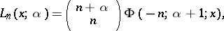
For classical orthogonal polynomials one has the generalized Rodrigues formula | For classical orthogonal polynomials one has the generalized Rodrigues formula | ||
| − | + | <table class="eq" style="width:100%;"> <tr><td valign="top" style="width:94%;text-align:center;"><img align="absmiddle" border="0" src="https://www.encyclopediaofmath.org/legacyimages/o/o070/o070340/o07034099.png" /></td> </tr></table> | |
| − | |||
| − | |||
| − | |||
| − | |||
| − | |||
| − | |||
| − | |||
| − | |||
| − | |||
| − | |||
| − | |||
| − | |||
| − | |||
| − | |||
| − | |||
| − | - | ||
| − | + | where <img align="absmiddle" border="0" src="https://www.encyclopediaofmath.org/legacyimages/o/o070/o070340/o070340100.png" /> is a normalization coefficient, and the differentiation formulas | |
| − | |||
| − | |||
| − | + | <table class="eq" style="width:100%;"> <tr><td valign="top" style="width:94%;text-align:center;"><img align="absmiddle" border="0" src="https://www.encyclopediaofmath.org/legacyimages/o/o070/o070340/o070340101.png" /></td> </tr></table> | |
| − | + | <table class="eq" style="width:100%;"> <tr><td valign="top" style="width:94%;text-align:center;"><img align="absmiddle" border="0" src="https://www.encyclopediaofmath.org/legacyimages/o/o070/o070340/o070340102.png" /></td> </tr></table> | |
| − | |||
| − | |||
| − | |||
| − | |||
| − | |||
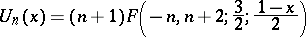
For particular cases of the classical orthogonal polynomials one has representations using the [[Hypergeometric function|hypergeometric function]] | For particular cases of the classical orthogonal polynomials one has representations using the [[Hypergeometric function|hypergeometric function]] | ||
| − | + | <table class="eq" style="width:100%;"> <tr><td valign="top" style="width:94%;text-align:center;"><img align="absmiddle" border="0" src="https://www.encyclopediaofmath.org/legacyimages/o/o070/o070340/o070340103.png" /></td> </tr></table> | |
| − | |||
| − | |||
| − | |||
| − | |||
| − | |||
| − | |||
| − | |||
| − | |||
| − | |||
| − | + | <table class="eq" style="width:100%;"> <tr><td valign="top" style="width:94%;text-align:center;"><img align="absmiddle" border="0" src="https://www.encyclopediaofmath.org/legacyimages/o/o070/o070340/o070340104.png" /></td> </tr></table> | |
| − | |||
| − | |||
| − | |||
| − | |||
| − | + | <table class="eq" style="width:100%;"> <tr><td valign="top" style="width:94%;text-align:center;"><img align="absmiddle" border="0" src="https://www.encyclopediaofmath.org/legacyimages/o/o070/o070340/o070340105.png" /></td> </tr></table> | |
| − | |||
| − | |||
| − | |||
| − | |||
| − | |||
| − | |||
| − | + | <table class="eq" style="width:100%;"> <tr><td valign="top" style="width:94%;text-align:center;"><img align="absmiddle" border="0" src="https://www.encyclopediaofmath.org/legacyimages/o/o070/o070340/o070340106.png" /></td> </tr></table> | |
| − | |||
| − | |||
| − | |||
| − | |||
| − | |||
| − | |||
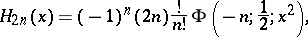
and using the [[Degenerate hypergeometric function|degenerate hypergeometric function]] | and using the [[Degenerate hypergeometric function|degenerate hypergeometric function]] | ||
| − | + | <table class="eq" style="width:100%;"> <tr><td valign="top" style="width:94%;text-align:center;"><img align="absmiddle" border="0" src="https://www.encyclopediaofmath.org/legacyimages/o/o070/o070340/o070340107.png" /></td> </tr></table> | |
| − | |||
| − | |||
| − | |||
| − | |||
| − | |||
| − | |||
| − | |||
| − | + | <table class="eq" style="width:100%;"> <tr><td valign="top" style="width:94%;text-align:center;"><img align="absmiddle" border="0" src="https://www.encyclopediaofmath.org/legacyimages/o/o070/o070340/o070340108.png" /></td> </tr></table> | |
| − | |||
| − | |||
| − | |||
| − | |||
| − | + | <table class="eq" style="width:100%;"> <tr><td valign="top" style="width:94%;text-align:center;"><img align="absmiddle" border="0" src="https://www.encyclopediaofmath.org/legacyimages/o/o070/o070340/o070340109.png" /></td> </tr></table> | |
| − | |||
| − | |||
| − | |||
| − | |||
| − | |||
Historically, the first orthogonal polynomials were the Legendre polynomials. Then came the Chebyshev polynomials, the general Jacobi polynomials, the Hermite and the Laguerre polynomials. All these classical orthogonal polynomials play an important role in many applied problems. | Historically, the first orthogonal polynomials were the Legendre polynomials. Then came the Chebyshev polynomials, the general Jacobi polynomials, the Hermite and the Laguerre polynomials. All these classical orthogonal polynomials play an important role in many applied problems. | ||
| Line 354: | Line 125: | ||
The general theory of orthogonal polynomials was formulated by P.L. Chebyshev. The basic research apparatus used was the [[Continued fraction|continued fraction]] expansion of the integral | The general theory of orthogonal polynomials was formulated by P.L. Chebyshev. The basic research apparatus used was the [[Continued fraction|continued fraction]] expansion of the integral | ||
| − | + | <table class="eq" style="width:100%;"> <tr><td valign="top" style="width:94%;text-align:center;"><img align="absmiddle" border="0" src="https://www.encyclopediaofmath.org/legacyimages/o/o070/o070340/o070340110.png" /></td> </tr></table> | |
| − | |||
| − | |||
| − | |||
| − | |||
| − | the denominators of the convergents of this continued fraction form a system of orthogonal polynomials on the interval | + | the denominators of the convergents of this continued fraction form a system of orthogonal polynomials on the interval <img align="absmiddle" border="0" src="https://www.encyclopediaofmath.org/legacyimages/o/o070/o070340/o070340111.png" /> with weight <img align="absmiddle" border="0" src="https://www.encyclopediaofmath.org/legacyimages/o/o070/o070340/o070340112.png" />. |
| − | with weight | ||
In the study of orthogonal polynomials, great attention is paid to their asymptotic properties, since the conditions of convergence of [[Fourier series in orthogonal polynomials|Fourier series in orthogonal polynomials]] depend on these properties. | In the study of orthogonal polynomials, great attention is paid to their asymptotic properties, since the conditions of convergence of [[Fourier series in orthogonal polynomials|Fourier series in orthogonal polynomials]] depend on these properties. | ||
| Line 367: | Line 133: | ||
The asymptotic properties of the classical orthogonal polynomials were first studied by V.A. Steklov in 1907 (see [[#References|[8]]]). He used and perfected the Liouville method, which was previously used in the study of solutions of the Sturm–Liouville equation. The Liouville–Steklov method was subsequently widely used, as a result of which the asymptotic properties of the Jacobi, Hermite and Laguerre orthogonal polynomials have been studied extensively. | The asymptotic properties of the classical orthogonal polynomials were first studied by V.A. Steklov in 1907 (see [[#References|[8]]]). He used and perfected the Liouville method, which was previously used in the study of solutions of the Sturm–Liouville equation. The Liouville–Steklov method was subsequently widely used, as a result of which the asymptotic properties of the Jacobi, Hermite and Laguerre orthogonal polynomials have been studied extensively. | ||
| − | In the general case of orthogonality on | + | In the general case of orthogonality on <img align="absmiddle" border="0" src="https://www.encyclopediaofmath.org/legacyimages/o/o070/o070340/o070340113.png" /> with arbitrary weight satisfying certain qualitative conditions, asymptotic formulas for orthogonal polynomials were first discovered by G. Szegö in 1920–1924. He introduced polynomials which were orthogonal on the circle, studied their basic properties and found an extremely important formula, representing polynomials orthogonal on <img align="absmiddle" border="0" src="https://www.encyclopediaofmath.org/legacyimages/o/o070/o070340/o070340114.png" /> by polynomials orthogonal on the circle. In his study of the asymptotic properties of polynomials orthogonal on the circle, Szegö developed a method based on a special generalization of the Fejér theorem on the representation of non-negative trigonometric polynomials by using methods and results of the theory of analytic functions. |
| − | with arbitrary weight satisfying certain qualitative conditions, asymptotic formulas for orthogonal polynomials were first discovered by G. Szegö in 1920–1924. He introduced polynomials which were orthogonal on the circle, studied their basic properties and found an extremely important formula, representing polynomials orthogonal on | ||
| − | by polynomials orthogonal on the circle. In his study of the asymptotic properties of polynomials orthogonal on the circle, Szegö developed a method based on a special generalization of the Fejér theorem on the representation of non-negative trigonometric polynomials by using methods and results of the theory of analytic functions. | ||
In 1930, S.N. Bernstein [S.N. Bernshtein] [[#References|[2]]], in his research on the asymptotic properties of orthogonal polynomials, used methods and results of the theory of approximation of functions. He examined the case of a weight function of the form | In 1930, S.N. Bernstein [S.N. Bernshtein] [[#References|[2]]], in his research on the asymptotic properties of orthogonal polynomials, used methods and results of the theory of approximation of functions. He examined the case of a weight function of the form | ||
| − | + | <table class="eq" style="width:100%;"> <tr><td valign="top" style="width:94%;text-align:center;"><img align="absmiddle" border="0" src="https://www.encyclopediaofmath.org/legacyimages/o/o070/o070340/o070340115.png" /></td> <td valign="top" style="width:5%;text-align:right;">(1)</td></tr></table> | |
| − | |||
| − | |||
| − | |||
| − | |||
| − | |||
| − | |||
| − | |||
| − | |||
| − | |||
| − | |||
| − | |||
| − | |||
| − | + | where the function <img align="absmiddle" border="0" src="https://www.encyclopediaofmath.org/legacyimages/o/o070/o070340/o070340116.png" />, called a trigonometric weight, satisfies the condition | |
| − | the function | ||
| − | |||
| − | |||
| − | |||
| − | + | <table class="eq" style="width:100%;"> <tr><td valign="top" style="width:94%;text-align:center;"><img align="absmiddle" border="0" src="https://www.encyclopediaofmath.org/legacyimages/o/o070/o070340/o070340117.png" /></td> </tr></table> | |
| − | |||
| − | |||
| − | , | + | If on the whole segment <img align="absmiddle" border="0" src="https://www.encyclopediaofmath.org/legacyimages/o/o070/o070340/o070340118.png" /> the function <img align="absmiddle" border="0" src="https://www.encyclopediaofmath.org/legacyimages/o/o070/o070340/o070340119.png" /> satisfies a Dini–Lipschitz condition of order <img align="absmiddle" border="0" src="https://www.encyclopediaofmath.org/legacyimages/o/o070/o070340/o070340120.png" />, where <img align="absmiddle" border="0" src="https://www.encyclopediaofmath.org/legacyimages/o/o070/o070340/o070340121.png" />, i.e. if |
| − | |||
| − | + | <table class="eq" style="width:100%;"> <tr><td valign="top" style="width:94%;text-align:center;"><img align="absmiddle" border="0" src="https://www.encyclopediaofmath.org/legacyimages/o/o070/o070340/o070340122.png" /></td> </tr></table> | |
| − | |||
| − | |||
| − | + | then for the polynomials <img align="absmiddle" border="0" src="https://www.encyclopediaofmath.org/legacyimages/o/o070/o070340/o070340123.png" /> orthonormal with weight (1) on the whole segment <img align="absmiddle" border="0" src="https://www.encyclopediaofmath.org/legacyimages/o/o070/o070340/o070340124.png" />, one has the asymptotic formula | |
| − | |||
| − | |||
| − | |||
| − | + | <table class="eq" style="width:100%;"> <tr><td valign="top" style="width:94%;text-align:center;"><img align="absmiddle" border="0" src="https://www.encyclopediaofmath.org/legacyimages/o/o070/o070340/o070340125.png" /></td> </tr></table> | |
| − | |||
| − | |||
| − | where | + | where <img align="absmiddle" border="0" src="https://www.encyclopediaofmath.org/legacyimages/o/o070/o070340/o070340126.png" /> and <img align="absmiddle" border="0" src="https://www.encyclopediaofmath.org/legacyimages/o/o070/o070340/o070340127.png" /> depends on <img align="absmiddle" border="0" src="https://www.encyclopediaofmath.org/legacyimages/o/o070/o070340/o070340128.png" />. |
| − | and | ||
| − | depends on | ||
| − | In the study of the convergence of Fourier series in orthogonal polynomials the question arises of the conditions of boundedness of the orthogonal polynomials, either at a single point, on a set | + | In the study of the convergence of Fourier series in orthogonal polynomials the question arises of the conditions of boundedness of the orthogonal polynomials, either at a single point, on a set <img align="absmiddle" border="0" src="https://www.encyclopediaofmath.org/legacyimages/o/o070/o070340/o070340129.png" /> or on the whole interval of orthogonality <img align="absmiddle" border="0" src="https://www.encyclopediaofmath.org/legacyimages/o/o070/o070340/o070340130.png" />, i.e. conditions are examined under which an inequality of the type |
| − | or on the whole interval of orthogonality | ||
| − | i.e. conditions are examined under which an inequality of the type | ||
| − | + | <table class="eq" style="width:100%;"> <tr><td valign="top" style="width:94%;text-align:center;"><img align="absmiddle" border="0" src="https://www.encyclopediaofmath.org/legacyimages/o/o070/o070340/o070340131.png" /></td> <td valign="top" style="width:5%;text-align:right;">(2)</td></tr></table> | |
| − | |||
| − | |||
| − | |||
| − | occurs. Steklov first posed this question in 1921. If the trigonometric weight | + | occurs. Steklov first posed this question in 1921. If the trigonometric weight <img align="absmiddle" border="0" src="https://www.encyclopediaofmath.org/legacyimages/o/o070/o070340/o070340132.png" /> is bounded away from zero on a set <img align="absmiddle" border="0" src="https://www.encyclopediaofmath.org/legacyimages/o/o070/o070340/o070340133.png" />, i.e. if |
| − | is bounded away from zero on a set | ||
| − | i.e. if | ||
| − | + | <table class="eq" style="width:100%;"> <tr><td valign="top" style="width:94%;text-align:center;"><img align="absmiddle" border="0" src="https://www.encyclopediaofmath.org/legacyimages/o/o070/o070340/o070340134.png" /></td> <td valign="top" style="width:5%;text-align:right;">(3)</td></tr></table> | |
| − | |||
| − | |||
| − | |||
and satisfies certain extra conditions, then the inequality (2) holds. In the general case, | and satisfies certain extra conditions, then the inequality (2) holds. In the general case, | ||
| − | + | <table class="eq" style="width:100%;"> <tr><td valign="top" style="width:94%;text-align:center;"><img align="absmiddle" border="0" src="https://www.encyclopediaofmath.org/legacyimages/o/o070/o070340/o070340135.png" /></td> <td valign="top" style="width:5%;text-align:right;">(4)</td></tr></table> | |
| − | |||
| − | |||
| − | |||
| − | |||
| − | |||
| − | |||
| − | |||
| − | + | follows from (3), when <img align="absmiddle" border="0" src="https://www.encyclopediaofmath.org/legacyimages/o/o070/o070340/o070340136.png" />, without extra conditions. | |
| − | |||
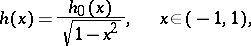
| − | + | The zeros of the weight function are singular points in the sense that the properties of the sequence <img align="absmiddle" border="0" src="https://www.encyclopediaofmath.org/legacyimages/o/o070/o070340/o070340137.png" /> are essentially different at the zeros and at other points of the interval of orthogonality. For example, let the weight function have the form | |
| − | |||
| − | + | <table class="eq" style="width:100%;"> <tr><td valign="top" style="width:94%;text-align:center;"><img align="absmiddle" border="0" src="https://www.encyclopediaofmath.org/legacyimages/o/o070/o070340/o070340138.png" /></td> </tr></table> | |
| − | |||
| − | |||
| − | |||
| − | |||
| − | If the function | + | If the function <img align="absmiddle" border="0" src="https://www.encyclopediaofmath.org/legacyimages/o/o070/o070340/o070340139.png" /> is positive and satisfies a Lipschitz condition on <img align="absmiddle" border="0" src="https://www.encyclopediaofmath.org/legacyimages/o/o070/o070340/o070340140.png" />, then the sequence <img align="absmiddle" border="0" src="https://www.encyclopediaofmath.org/legacyimages/o/o070/o070340/o070340141.png" /> is bounded on every segment <img align="absmiddle" border="0" src="https://www.encyclopediaofmath.org/legacyimages/o/o070/o070340/o070340142.png" /> which does not contain the points <img align="absmiddle" border="0" src="https://www.encyclopediaofmath.org/legacyimages/o/o070/o070340/o070340143.png" />, while the inequalities |
| − | is positive and satisfies a Lipschitz condition on | ||
| − | then the sequence | ||
| − | is bounded on every segment | ||
| − | which does not contain the points | ||
| − | while the inequalities | ||
| − | + | <table class="eq" style="width:100%;"> <tr><td valign="top" style="width:94%;text-align:center;"><img align="absmiddle" border="0" src="https://www.encyclopediaofmath.org/legacyimages/o/o070/o070340/o070340144.png" /></td> </tr></table> | |
| − | |||
| − | |||
| − | |||
hold at the zeros. | hold at the zeros. | ||
| Line 474: | Line 179: | ||
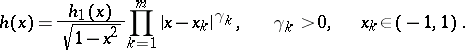
The case where the zeros of the weight function are positioned at the ends of the segment of orthogonality was studied by Bernstein [[#References|[2]]]. One of the results is that if the weight function has the form | The case where the zeros of the weight function are positioned at the ends of the segment of orthogonality was studied by Bernstein [[#References|[2]]]. One of the results is that if the weight function has the form | ||
| − | + | <table class="eq" style="width:100%;"> <tr><td valign="top" style="width:94%;text-align:center;"><img align="absmiddle" border="0" src="https://www.encyclopediaofmath.org/legacyimages/o/o070/o070340/o070340145.png" /></td> </tr></table> | |
| − | |||
| − | |||
| − | |||
| − | where the function | + | where the function <img align="absmiddle" border="0" src="https://www.encyclopediaofmath.org/legacyimages/o/o070/o070340/o070340146.png" /> is positive and satisfies a Lipschitz condition, then for <img align="absmiddle" border="0" src="https://www.encyclopediaofmath.org/legacyimages/o/o070/o070340/o070340147.png" />, <img align="absmiddle" border="0" src="https://www.encyclopediaofmath.org/legacyimages/o/o070/o070340/o070340148.png" />, the orthogonal polynomials permit the weighted estimation |
| − | is positive and satisfies a Lipschitz condition, then for | ||
| − | |||
| − | the orthogonal polynomials permit the weighted estimation | ||
| − | + | <table class="eq" style="width:100%;"> <tr><td valign="top" style="width:94%;text-align:center;"><img align="absmiddle" border="0" src="https://www.encyclopediaofmath.org/legacyimages/o/o070/o070340/o070340149.png" /></td> </tr></table> | |
| − | |||
| − | |||
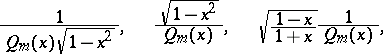
| − | while at the points | + | while at the points <img align="absmiddle" border="0" src="https://www.encyclopediaofmath.org/legacyimages/o/o070/o070340/o070340150.png" /> they increase at a rate <img align="absmiddle" border="0" src="https://www.encyclopediaofmath.org/legacyimages/o/o070/o070340/o070340151.png" /> and <img align="absmiddle" border="0" src="https://www.encyclopediaofmath.org/legacyimages/o/o070/o070340/o070340152.png" />, respectively. |
| − | they increase at a rate | ||
| − | and | ||
| − | respectively. | ||
| − | In the theory of orthogonal polynomials, so-called comparison theorems are often studied. One such is the Korous comparison theorem: If the polynomials | + | In the theory of orthogonal polynomials, so-called comparison theorems are often studied. One such is the Korous comparison theorem: If the polynomials <img align="absmiddle" border="0" src="https://www.encyclopediaofmath.org/legacyimages/o/o070/o070340/o070340153.png" /> are orthogonal with weight <img align="absmiddle" border="0" src="https://www.encyclopediaofmath.org/legacyimages/o/o070/o070340/o070340154.png" /> on the segment <img align="absmiddle" border="0" src="https://www.encyclopediaofmath.org/legacyimages/o/o070/o070340/o070340155.png" /> and are uniformly bounded on a set <img align="absmiddle" border="0" src="https://www.encyclopediaofmath.org/legacyimages/o/o070/o070340/o070340156.png" />, then the polynomials <img align="absmiddle" border="0" src="https://www.encyclopediaofmath.org/legacyimages/o/o070/o070340/o070340157.png" />, orthogonal with weight <img align="absmiddle" border="0" src="https://www.encyclopediaofmath.org/legacyimages/o/o070/o070340/o070340158.png" />, are also bounded on this set, provided <img align="absmiddle" border="0" src="https://www.encyclopediaofmath.org/legacyimages/o/o070/o070340/o070340159.png" /> is positive and satisfies a Lipschitz condition of order <img align="absmiddle" border="0" src="https://www.encyclopediaofmath.org/legacyimages/o/o070/o070340/o070340160.png" /> on <img align="absmiddle" border="0" src="https://www.encyclopediaofmath.org/legacyimages/o/o070/o070340/o070340161.png" />. Similarly, given certain conditions on <img align="absmiddle" border="0" src="https://www.encyclopediaofmath.org/legacyimages/o/o070/o070340/o070340162.png" />, asymptotic formulas or other asymptotic properties can be transferred from the system <img align="absmiddle" border="0" src="https://www.encyclopediaofmath.org/legacyimages/o/o070/o070340/o070340163.png" /> to the system <img align="absmiddle" border="0" src="https://www.encyclopediaofmath.org/legacyimages/o/o070/o070340/o070340164.png" />. Moreover, if <img align="absmiddle" border="0" src="https://www.encyclopediaofmath.org/legacyimages/o/o070/o070340/o070340165.png" /> is a non-negative polynomial of degree <img align="absmiddle" border="0" src="https://www.encyclopediaofmath.org/legacyimages/o/o070/o070340/o070340166.png" /> on <img align="absmiddle" border="0" src="https://www.encyclopediaofmath.org/legacyimages/o/o070/o070340/o070340167.png" />, then the polynomials <img align="absmiddle" border="0" src="https://www.encyclopediaofmath.org/legacyimages/o/o070/o070340/o070340168.png" /> can be represented by the polynomials <img align="absmiddle" border="0" src="https://www.encyclopediaofmath.org/legacyimages/o/o070/o070340/o070340169.png" /> using determinants of order <img align="absmiddle" border="0" src="https://www.encyclopediaofmath.org/legacyimages/o/o070/o070340/o070340170.png" /> (see [[#References|[8]]]). Effective formulas for orthogonal polynomials have also been obtained for weight functions of the form |
| − | are orthogonal with weight | ||
| − | on the segment | ||
| − | and are uniformly bounded on a set | ||
| − | then the polynomials | ||
| − | orthogonal with weight | ||
| − | are also bounded on this set, provided | ||
| − | is positive and satisfies a Lipschitz condition of order | ||
| − | on | ||
| − | Similarly, given certain conditions on | ||
| − | asymptotic formulas or other asymptotic properties can be transferred from the system | ||
| − | to the system | ||
| − | Moreover, if | ||
| − | is a non-negative polynomial of degree | ||
| − | on | ||
| − | then the polynomials | ||
| − | can be represented by the polynomials | ||
| − | using determinants of order | ||
| − | see [[#References|[8]]]). Effective formulas for orthogonal polynomials have also been obtained for weight functions of the form | ||
| − | + | <table class="eq" style="width:100%;"> <tr><td valign="top" style="width:94%;text-align:center;"><img align="absmiddle" border="0" src="https://www.encyclopediaofmath.org/legacyimages/o/o070/o070340/o070340171.png" /></td> </tr></table> | |
| − | + | where <img align="absmiddle" border="0" src="https://www.encyclopediaofmath.org/legacyimages/o/o070/o070340/o070340172.png" /> is an arbitrary positive polynomial on <img align="absmiddle" border="0" src="https://www.encyclopediaofmath.org/legacyimages/o/o070/o070340/o070340173.png" /> (see [[#References|[8]]]). In most cases, the calculation of orthogonal polynomials with arbitrary weight is difficult for large numbers <img align="absmiddle" border="0" src="https://www.encyclopediaofmath.org/legacyimages/o/o070/o070340/o070340174.png" />. | |
| − | |||
| − | + | ====References==== | |
| − | , | + | <table><TR><TD valign="top">[1]</TD> <TD valign="top"> P.L. Chebyshev, "Complete collected works" , '''2''' , Moscow-Leningrad (1947) pp. 103–126; 314–334; 335–341; 357–374 (In Russian)</TD></TR><TR><TD valign="top">[2]</TD> <TD valign="top"> S.N. Bernshtein, "Collected works" , '''2''' , Moscow (1954) pp. 7–106 (In Russian)</TD></TR><TR><TD valign="top">[3]</TD> <TD valign="top"> Ya.L. Geronimus, "Orthogonal polynomials" ''Transl. Amer. Math. Soc.'' , '''108''' (1977) pp. 37–130</TD></TR><TR><TD valign="top">[4]</TD> <TD valign="top"> P.K. Suetin, "Classical orthogonal polynomials" , Moscow (1979) (In Russian)</TD></TR><TR><TD valign="top">[5]</TD> <TD valign="top"> V.B. Uvarov, "Special functions of mathematical physics" , Birkhäuser (1988) (Translated from Russian)</TD></TR><TR><TD valign="top">[6]</TD> <TD valign="top"> H. Bateman (ed.) A. Erdélyi (ed.) et al. (ed.) , ''Higher transcendental functions'' , '''2. Bessel functions, parabolic cylinder functions, orthogonal polynomials''' , McGraw-Hill (1953)</TD></TR><TR><TD valign="top">[7]</TD> <TD valign="top"> D. Jackson, "Fourier series and orthogonal polynomials" , ''Carus Math. Monogr.'' , '''6''' , Math. Assoc. Amer. (1971)</TD></TR><TR><TD valign="top">[8]</TD> <TD valign="top"> G. Szegö, "Orthogonal polynomials" , Amer. Math. Soc. (1975)</TD></TR><TR><TD valign="top">[9]</TD> <TD valign="top"> , ''Guide to special functions'' , Moscow (1979) (In Russian; translated from English)</TD></TR><TR><TD valign="top">[10]</TD> <TD valign="top"> J.A. Shohat, E. Hille, J.L. Walsh, "A bibliography on orthogonal polynomials" , Nat. Acad. Sci. USA (1940)</TD></TR></table> |
| − | |||
| − | |||
| − | |||
| − | |||
| − | , | ||
| − | |||
| − | |||
| − | |||
| − | |||
| − | |||
| − | |||
====Comments==== | ====Comments==== | ||
Revision as of 14:52, 7 June 2020
A system of polynomials  which satisfy the condition of orthogonality
 |
whereby the degree of every polynomial  is equal to its index
  , and the weight function (weight)
  on the interval
  or (when
  and
and  are finite) on
  . Orthogonal polynomials are said to be orthonormalized, and are denoted by
  , if every polynomial has positive leading coefficient and if the normalizing condition
 |
is fulfilled. If the leading coefficient of each polynomial is equal to 1, then the system of orthogonal polynomials is denoted by  .
.
The system of orthogonal polynomials  is uniquely defined if the weight function (differential weight)
  is Lebesgue integrable on
  , is not equivalent to zero and, in the case of an unbounded interval
  , has finite moments
 |
Instead of a differential weight  , an integral weight
  can be examined, where
  is a bounded non-decreasing function with an infinite set of points of growth (in this case, the integral in the condition of orthogonality is understood in the Lebesgue–Stieltjes sense).
For the polynomial  of degree
  to be part of the system
  with weight
  , it is necessary and sufficient that, for any polynomial
  of degree
  , the condition
 |
is fulfilled. If the interval of orthogonality  is symmetric with respect to the origin and the weight function
  is even, then every polynomial
  contains only those degrees of
  which have the parity of the number
  , i.e. one has the identity
 |
The zeros of orthogonal polynomials in the case of the interval  are all real, different and distributed within
  , while between two neighbouring zeros of the polynomial
  there is one zero of the polynomial
  . Zeros of orthogonal polynomials are often used as interpolation points and in quadrature formulas.
Any three consecutive polynomials of a system of orthogonal polynomials are related by a recurrence formula
 |
where
 |
 |
 |
 |
 |
The number  is a normalization factor of the polynomial
  , such that the system
  is orthonormalized, i.e.
 |
For orthogonal polynomials one has the Christoffel–Darboux formula:
 |
 |
Orthogonal polynomials are represented in terms of the moments  of the weight function
  by the formula
 |
where
 |
while the determinant  is obtained from
  by cancelling the last row and column and
  is defined in the same way from
  .
.
On a set of polynomials  of degree
  with leading coefficient equal to one, the minimum of the functional
 |
is achieved if and only if
 |
moreover, this minimum is equal to  .
.
If the polynomials  are orthonormal with weight
  on the segment
  , then when
  , the polynomials
 |
are orthonormal with weight  on the segment
  which transfers to the segment
  as a result of the linear transformation
  . For this reason, when studying the asymptotic properties of orthogonal polynomials, the case of the standard segment
  is considered first, while the results thus obtained cover other cases as well.
The most important orthogonal polynomials encountered in solving boundary problems of mathematical physics are the so-called classical orthogonal polynomials: the Laguerre polynomials  (for which
 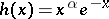 ,
,  , and with interval of orthogonality
  ); the Hermite polynomials
  (for which
  , and with interval of orthogonality
  ); the Jacobi polynomials
  (for which
  ,
,  ,
,  , and with interval of orthogonality
  ) and their particular cases: the ultraspherical polynomials, or Gegenbauer polynomials,
  (for which
  ), the Legendre polynomials
  (for which
  ), the Chebyshev polynomials of the first kind
  (for which
  ) and of the second kind
  (for which
  ).
).
The weight function  of the classical orthogonal polynomials
  satisfies the Pearson differential equation
 |
whereby, at the ends of the interval of orthogonality, the conditions
 |
are fulfilled.
The polynomial  satisfies the differential equation
 |
For classical orthogonal polynomials one has the generalized Rodrigues formula
 |
where  is a normalization coefficient, and the differentiation formulas
 |
 |
For particular cases of the classical orthogonal polynomials one has representations using the hypergeometric function
 |
 |
 |
 |
and using the degenerate hypergeometric function
 |
 |
 |
Historically, the first orthogonal polynomials were the Legendre polynomials. Then came the Chebyshev polynomials, the general Jacobi polynomials, the Hermite and the Laguerre polynomials. All these classical orthogonal polynomials play an important role in many applied problems.
The general theory of orthogonal polynomials was formulated by P.L. Chebyshev. The basic research apparatus used was the continued fraction expansion of the integral
 |
the denominators of the convergents of this continued fraction form a system of orthogonal polynomials on the interval  with weight
  .
.
In the study of orthogonal polynomials, great attention is paid to their asymptotic properties, since the conditions of convergence of Fourier series in orthogonal polynomials depend on these properties.
The asymptotic properties of the classical orthogonal polynomials were first studied by V.A. Steklov in 1907 (see [8]). He used and perfected the Liouville method, which was previously used in the study of solutions of the Sturm–Liouville equation. The Liouville–Steklov method was subsequently widely used, as a result of which the asymptotic properties of the Jacobi, Hermite and Laguerre orthogonal polynomials have been studied extensively.
In the general case of orthogonality on  with arbitrary weight satisfying certain qualitative conditions, asymptotic formulas for orthogonal polynomials were first discovered by G. Szegö in 1920–1924. He introduced polynomials which were orthogonal on the circle, studied their basic properties and found an extremely important formula, representing polynomials orthogonal on
  by polynomials orthogonal on the circle. In his study of the asymptotic properties of polynomials orthogonal on the circle, Szegö developed a method based on a special generalization of the Fejér theorem on the representation of non-negative trigonometric polynomials by using methods and results of the theory of analytic functions.
In 1930, S.N. Bernstein [S.N. Bernshtein] [2], in his research on the asymptotic properties of orthogonal polynomials, used methods and results of the theory of approximation of functions. He examined the case of a weight function of the form
 | (1) |
where the function  , called a trigonometric weight, satisfies the condition
 |
If on the whole segment  the function
  satisfies a Dini–Lipschitz condition of order
  , where
  , i.e. if
 |
then for the polynomials  orthonormal with weight (1) on the whole segment
  , one has the asymptotic formula
 |
where  and
and  depends on
  .
.
In the study of the convergence of Fourier series in orthogonal polynomials the question arises of the conditions of boundedness of the orthogonal polynomials, either at a single point, on a set  or on the whole interval of orthogonality
  , i.e. conditions are examined under which an inequality of the type
 | (2) |
occurs. Steklov first posed this question in 1921. If the trigonometric weight  is bounded away from zero on a set
  , i.e. if
 | (3) |
and satisfies certain extra conditions, then the inequality (2) holds. In the general case,
 | (4) |
follows from (3), when  , without extra conditions.
The zeros of the weight function are singular points in the sense that the properties of the sequence  are essentially different at the zeros and at other points of the interval of orthogonality. For example, let the weight function have the form
 |
If the function  is positive and satisfies a Lipschitz condition on
  , then the sequence
  is bounded on every segment
 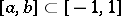 which does not contain the points
  , while the inequalities
 |
hold at the zeros.
The case where the zeros of the weight function are positioned at the ends of the segment of orthogonality was studied by Bernstein [2]. One of the results is that if the weight function has the form
 |
where the function  is positive and satisfies a Lipschitz condition, then for
  ,
,  , the orthogonal polynomials permit the weighted estimation
 |
while at the points  they increase at a rate
  and
and  , respectively.
In the theory of orthogonal polynomials, so-called comparison theorems are often studied. One such is the Korous comparison theorem: If the polynomials  are orthogonal with weight
  on the segment
  and are uniformly bounded on a set
  , then the polynomials
  , orthogonal with weight
  , are also bounded on this set, provided
  is positive and satisfies a Lipschitz condition of order
  on
on  . Similarly, given certain conditions on
  , asymptotic formulas or other asymptotic properties can be transferred from the system
  to the system
  . Moreover, if
  is a non-negative polynomial of degree
  on
on  , then the polynomials
  can be represented by the polynomials
  using determinants of order
  (see [8]). Effective formulas for orthogonal polynomials have also been obtained for weight functions of the form
 |
where  is an arbitrary positive polynomial on
  (see [8]). In most cases, the calculation of orthogonal polynomials with arbitrary weight is difficult for large numbers
  .
.
References
| [1] | P.L. Chebyshev, "Complete collected works" , 2 , Moscow-Leningrad (1947) pp. 103–126; 314–334; 335–341; 357–374 (In Russian) |
| [2] | S.N. Bernshtein, "Collected works" , 2 , Moscow (1954) pp. 7–106 (In Russian) |
| [3] | Ya.L. Geronimus, "Orthogonal polynomials" Transl. Amer. Math. Soc. , 108 (1977) pp. 37–130 |
| [4] | P.K. Suetin, "Classical orthogonal polynomials" , Moscow (1979) (In Russian) |
| [5] | V.B. Uvarov, "Special functions of mathematical physics" , Birkhäuser (1988) (Translated from Russian) |
| [6] | H. Bateman (ed.) A. Erdélyi (ed.) et al. (ed.) , Higher transcendental functions , 2. Bessel functions, parabolic cylinder functions, orthogonal polynomials , McGraw-Hill (1953) |
| [7] | D. Jackson, "Fourier series and orthogonal polynomials" , Carus Math. Monogr. , 6 , Math. Assoc. Amer. (1971) |
| [8] | G. Szegö, "Orthogonal polynomials" , Amer. Math. Soc. (1975) |
| [9] | , Guide to special functions , Moscow (1979) (In Russian; translated from English) |
| [10] | J.A. Shohat, E. Hille, J.L. Walsh, "A bibliography on orthogonal polynomials" , Nat. Acad. Sci. USA (1940) |
Comments
See also Fourier series in orthogonal polynomials. Two other textbooks are [a3] and [a2]. See [a1] for some more information on the history of the classical orthogonal polynomials. Regarding the asymptotic properties of the classical orthogonal polynomials it should be observed that many workers (P.S. Laplace, E. Heine, G. Darboux, T.J. Stieltjes, E. Hilb, etc.) preceded Stekov, but he was the first to adapt Liouville's method.
See [a5] for state-of-the-art surveys of many aspects of orthogonal polynomials. In particular, the general theory of orthogonal polynomials with weight functions on unbounded intervals has made big progress, see also [a4].
References
| [a1] | R.A. Askey, "Discussion of Szegö's paper "An outline of the history of orthogonal polynomials" " R.A. Askey (ed.) , G.P. Szegö: Collected Works , 3 , Birkhäuser (1982) pp. 866–869 |
| [a2] | T.S. Chihara, "An introduction to orthogonal polynomials" , Gordon & Breach (1978) |
| [a3] | G. Freud, "Orthogonal polynomials" , Pergamon (1971) (Translated from German) |
| [a4] | D.S. Lubinsky, "A survey of general orthogonal polynomials for weights on finite and infinite intervals" Acta Applic. Math. , 10 (1987) pp. 237–296 |
| [a5] | P. Nevai (ed.) , Orthogonal polynomials: theory and practice , Kluwer (1990) |
Orthogonal polynomials. Encyclopedia of Mathematics. URL: http://encyclopediaofmath.org/index.php?title=Orthogonal_polynomials&oldid=48076