Large-particle method
A method for computing compressible flows of a continuous medium [1]. The method is based on splitting the original differential equations in accordance with the physical processes they represent (see [3]). It can be used to solve systems of evolution equations. The procedure may establish the existence of steady-state solutions. The large-particle method is a development of Harlow's method of "particle-in-cell" .
The method is widely used to investigate aerodynamic flows, diffraction problems, transonic flows, interaction phenomena of radiation and matter, etc.
The difference scheme of the method may be illustrated by considering the motion of an ideal compressible gas (the continuity, the momentum and the energy equation):
$$ \tag{1 } \left . \begin{array}{c} \frac{\partial \rho }{\partial t } + \mathop{\rm div} ( \rho \mathbf v ) = 0, \\ \frac{\partial \rho u _ {i} }{\partial t } + \mathop{\rm div} ( \rho \mathbf v u _ {i} ) + \frac{\partial P }{\partial x _ {i} } = 0, \\ \frac{\partial \rho E }{\partial t } + \mathop{\rm div} ( \rho E \mathbf v ) + \mathop{\rm div} ( P \mathbf v ) = 0. \\ \end{array} \right \} $$
Here $ x _ {i} = \{ x, y, z \} $, $ t $ denotes time, $ \rho $ the density, $ \mathbf v = \{ u _ {i} \} = \{ u , v, w \} $ the velocity, $ E $ the total specific energy, and $ P $ the pressure. To close the system (1) one uses the equation of state
$$ P = P ( \rho , J), $$
where
$$ J = E - { \frac{1}{2} } | \mathbf v | ^ {2} $$
is the specific internal energy.
The solution process for an evolution system (1) is divided into three chronological stages, each of which consists of three steps: an Eulerian, a Lagrangian and a final one. One first considers the variation of the internal state of a subsystem — a "large particle" (Eulerian step), and then — the motion of this subsystem with the interior state of the subsystem left unchanged (Lagrangian and final steps).
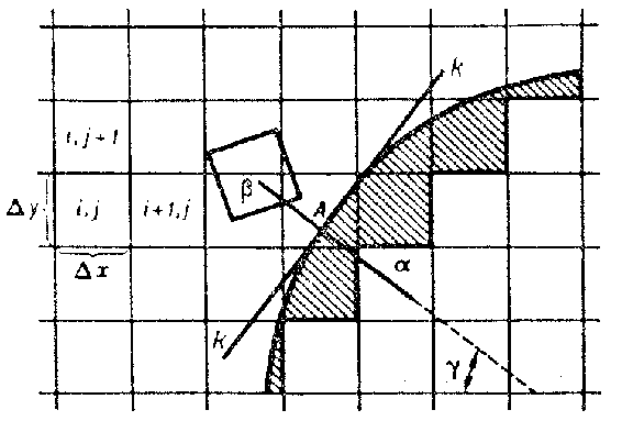
Figure: l057570a
Eulerian step. The domain of integration is covered by a stationary (Eulerian) difference grid of arbitrary form (to abbreviate the exposition, a rectangular grid in a two-dimensional (planar) domain is considered, see Fig.). At this step of the calculation only quantities relating to the cell as a whole are varied, while the fluid is assumed to be momentarily constrained. For this reason, convective terms such as $ \mathop{\rm div} ( \psi \rho \mathbf v ) $, $ \psi = ( 1, u , v , E) $, corresponding to translational effects, are dropped from the equations (1). In the remaining equations of (1), $ \rho $ is brought forward outside the differentiation symbol, and the equations (1) are solved for the derivatives of $ u $, $ v $ and $ E $ with respect to the time:
$$ \tag{2 } \rho \frac{\partial u }{\partial t } + \frac{\partial P }{\partial x } = 0,\ \ \rho \frac{\partial v }{\partial t } + \frac{\partial P }{\partial y } = 0, $$
$$ \rho \frac{\partial E }{\partial t } + \mathop{\rm div} ( P \mathbf v ) = 0. $$
An elementary finite-difference approximation (central differences) yields the following expressions:
$$ \widetilde{u} {} _ {i, j } ^ {n} = \ u _ {i, j } ^ {n} - \frac{P _ {i + 1/2, j } ^ {n} - P _ {i - 1/2, j } ^ {n} }{\Delta x } \frac{\Delta t }{\rho _ {i, j } ^ {n} } , $$
$$ \widetilde{v} {} _ {i, j } ^ {n} = v _ {i, j } ^ {n} - \frac{P _ {i, j + 1/2 } ^ {n} - P _ {i, j - 1/2 } ^ {n} }{\Delta y } \frac{\Delta t }{\rho _ {i, j } ^ {n} } , $$
$$ \widetilde{E} {} _ {i,j} ^ {n} = E _ {i,j} ^ {n} - $$
$$ - \left [ \frac{P _ {i + 1/2, j } ^ {n} \widetilde{u} {} _ {i + 1/2 , j } ^ {n} - P _ {i - 1/2 , j } ^ {n} u tilde {} _ {i - 1/2 , j } ^ {n} }{\Delta x } \right . + $$
$$ + \left . \frac{P _ {i, j + 1/2 } ^ {n} \widetilde{v} {} _ {i, j + 1/2 } ^ {n} - P _ {i, j + 1/2 } ^ {n} v tilde {} _ {i, j - 1/2 } ^ {n} }{\Delta y } \right ] \frac{\Delta t }{\rho _ {i, j } ^ {n} } . $$
Quantities with fractional subscripts relate to cell boundaries, e.g.
$$ u _ {i + 1/2, j } ^ {n} = \ \frac{u _ {i, j } ^ {n} + u _ {i + 1, j } ^ {n} }{2} , P _ {i - 1/2, j } ^ {n} = \ \frac{P _ {i - 1, j } ^ {n} + P _ {i, j } ^ {n} }{2} , . . . ; $$
$ \widetilde{u} $, $ \widetilde{v} $, $ \widetilde{E} $ are intermediate values of the flow parameters, obtained on the assumption that the field $ \rho $ is "frozen" in the layer $ t ^ {n} + \Delta t $. Although the scheme of the Eulerian step in this form is unstable, the scheme as a whole is stable if the next steps are suitably formulated. The Eulerian step may be made stable, for example, by introducing elements of the integral-relation method. When this is done the integrands are approximated in the direction parallel to the axes of the body (see Fig.), i.e. as in scheme 1 of the integral-relation method: The original system of equations is taken to be in integral form, and the following integrals are approximated:
$$ f = \int\limits _ { V } \rho u d \tau ,\ \ \theta = \int\limits _ { V } \rho v d \tau ,\ \ \psi = \int\limits _ { V } \rho E d \tau . $$
Lagrangian step. Now one calculates the mass flow through the cell boundaries at time $ t ^ {n} + \Delta t $. It is assumed throughout that the mass of the large particle is in motion only owing to the velocity component normal to the boundary. Thus,
$$ \Delta M _ {i + 1/2, j } ^ {n} = \ \langle \rho _ {i + 1/2, j } ^ {n} \rangle \langle u _ {i + 1/2, j } ^ {n} \rangle \Delta y \Delta t, $$
etc. The angular brackets define the parameters $ \rho $ and $ u $ at the cell boundaries. The choice of these quantities is of paramount importance, since it strongly influences the stability and accuracy of the computation. Various difference representations are possible for $ \Delta M ^ {n} $: of different orders of accuracy, with or without allowance for the flow direction, central differences, ZIP-approximations, etc. The momentum (energy) flows are equal to the products of $ \Delta M ^ {n} $ and the corresponding value of the velocity (total specific energy). Approximations have been worked out not only for mass flows, but also for momentum and energy flows.
Final step. At this step one finds the final fields of the Eulerian flow parameters at the time $ t ^ {n + 1 } = t ^ {n} + \Delta t $. The equations of this step are conservation laws for the mass $ M $, the momentum $ \mathbf p $ and the total energy $ E $, relating to a given cell (large particle) in finite-difference form $ M ^ {n+ 1 } = M ^ {n} + \sum \Delta M ^ {n} $, $ \mathbf p ^ {n + 1 } = \mathbf p ^ {n} + \sum \Delta \mathbf p ^ {n} $, $ E ^ {n + 1 } = E ^ {n} + \sum \Delta E ^ {n} $. The final values of the flow parameters $ \rho $, $ X = \{ u , v, E \} $ in the next time layer are computed according to the following formulas (the direction of the flow is from left to right and upwards):
$$ \rho _ {i, j } ^ {n + 1 } = \ \rho _ {i, j } ^ {n} + $$
$$ + \frac{\Delta M _ {i - 1/2, j } ^ {n} + \Delta M _ {i, j - 1/2 } ^ {n} - \Delta M _ {i, j + 1/2 } ^ {n} - \Delta M _ {i + 1/2, j } ^ {n} }{\Delta x \Delta y } , $$
$$ X _ {i, j } ^ {n + 1 } = $$
$$ = \ \frac{\rho _ {i, j } ^ {n} }{\rho _ {i, j } ^ {n + 1 } } \widetilde{X} {} _ {i, j } ^ {n} + \frac{\widetilde{X} {} _ {i - 1, j } ^ {n} \Delta M _ {i - 1/2, j } ^ {n} + \widetilde{X} {} _ {i, j - 1 } ^ {n} \Delta M _ {i, j - 1/2 } ^ {n} }{\rho _ {i, j } ^ {n + 1 } \Delta x \Delta y } - $$
$$ - \frac{\widetilde{X} {} _ {i, j } ^ {n} \Delta M _ {i + 1/2, j } ^ {n} + \widetilde{X} {} _ {i, j } ^ {n} \Delta M _ {i, j + 1/2 } ^ {n} }{\rho _ {i, j } ^ {n + 1 } \Delta x \Delta y } . $$
The conservativity and total divergency of the difference scheme (divergent-conservative scheme) are guaranteed by the equation for the total energy $ E $. At the final step (when a discrete model of the medium is being used) one should carry out an additional calculation of the density; this smoothens out fluctuations and increases the accuracy of the computations. Combining the different representations of the steps, one obtains a series of difference schemes; this series, which constitutes the large-particle method, may be used for a broad range of numerical experiments.
The large-particle method may be interpreted from various points of view: the splitting method, the mixed Euler–Lagrange method, computation in local Lagrangian coordinates (Eulerian step) with scaling on the previous grid (Lagrangian and final steps), the difference notation for conservation laws for a fluid element (large particle), and the Eulerian difference scheme.
The boundary conditions are formulated by introducing series of fictitious cells (so that every computation point becomes an interior point and the same algorithm is maintained for all cells). One layer is sufficient for the first-order approximation scheme, two layers are sufficient for the second order, etc. For example, consider the problem of calculating the flow around axially-symmetric or plane bodies with generators of arbitrary form (see Fig.). The above difference formulas are valid for interior cells of the field, surrounded on all sides by fluid, and for cells bordering on the solid body, the contour of which coincides with the cell boundaries.
There are two possible approaches to the computation of flow around bodies using finite-difference methods: A computation in the coordinates $ s $, $ n $; or an introduction of fractional cells (see [2]). In the first case one encounters difficulties in treating bodies with fractures and concavities. The second approach is free from these disadvantages.
In the case of fractional cells, the boundary conditions on the body are formulated, as in the case of whole cells, by introducing fictitious cells. Inside the body one has a layer of fictitious cells bordering on the fractional cells. To determine the parameters of the gas in these fictitious cells, one constructs the normal from the centre of each fictitious cell $ \alpha $ to the contour of the body; if $ A $ is the point of intersection of the normal and the contour, let $ k $ be the tangent at $ A $( see Fig.). Now let $ \beta $ be the cell in the field of the flow, symmetric to $ \alpha $ with respect to $ k $. The gas-dynamical parameters $ g $ in $ \beta $ are determined by "weighting" , $ g _ \beta = \sum _ {i} S _ {\beta _ {i} } g _ {i} $( $ \sum _ {i} S _ {\beta _ {i} } = 1 $), where the summation is over those cells $ i $ such that part of the area $ S _ {\beta _ {i} } $ lies in the cell $ \beta $. In order to formulate conditions stating that the body is impermeable, one more parameter has to be determined for each fictitious cell — $ \gamma $, the inclination of the radius vector that cuts the body contour at $ A $. If one is using adhesion conditions (both velocity components change sign across the surface of the body), this additional determination of $ \gamma $ is not necessary. The parameters of the gas in the fictitious cell $ \alpha $ then are
$$ \left \{ \begin{array}{c} \rho \\ E \end{array} \right \} _ \alpha = \ \sum S _ {\beta _ {i} } \left \{ \begin{array}{c} \rho \\ E \end{array} \right \} _ {i} ,\ \ \left \{ \begin{array}{c} u \\ v \end{array} \right \} _ \alpha = \ - \sum S _ {\beta _ {i} } \left \{ \begin{array}{c} u \\ v \end{array} \right \} _ {i} . $$
The boundary conditions for a body whose contour coincides with the cell boundaries constitute a particular case of the boundary conditions presented here.
For each fractional cell (see Fig.) one needs to know five geometrical characteristics: $ A _ {i - 1/2, j } $, $ A _ {i, j - 1/2 } $, $ A _ {i+ 1/2, j } $, $ A _ {i, j + 1/2 } $, and $ f _ {i, j } $, where $ f _ {i, j } $ is the ratio of the volume of the fractional cell to the volume $ \Delta x \Delta y $ of the whole cell, $ A _ {i - 1/2, j } $ is the fraction of the area of the side $ ( i - 1/2, j ) $ open for the flow, etc.
The existence of a solid boundary within a cell implies two special features: It shifts the mass centre from the geometrical centre of the cell, bringing it closer to the boundary; and it reduces the actual size of the cell. With regard to both whole and fractional cells, all flow parameters refer to the centre of mass. It is between the centres of mass that one interpolates the gas-dynamical functions. In whole cells, the centre of mass is either identical to the geometrical centre of the cell (the plane Cartesian coordinate system) or near it (the cylindrical coordinate system). In actual computations, the difference, even for the row of cells along the axis, is at most $ 0.2 \Delta r $. This does not substantially distort the results of the computations. If fractional cells are introduced in an appropriate way, the displacement of the centre of mass relative to the geometrical centre does not increase this error. The reduction in the effective size of the cells is a more serious matter. To avoid violation of the stability condition $ c ( \Delta t/ \Delta \lambda ) < 1 $, where $ \lambda $ is $ x $ or $ y $, those cells with $ f < f _ {\textrm{ min }.st } $ should be combined with adjacent whole cells within the flow, and the resulting combinations should be computed using the formulas for fractional cells. In this case, the geometrical dimensions of an enlarged cell will not be less than those of a whole cell: $ A _ {i - 1/2, j } \geq 1 $, $ A _ {i, j - 1/2 } \geq 1 \dots f _ {i, j } > 1 $, so that the question of the stability of fractional cells is eliminated.
In the planar case, the geometrical characteristics of fractional cells may be determined by direct measurement. In the axially-symmetric case one needs an additional computation, incorporating the distance of each fractional cell from the axis of symmetry. The difference formulas for fractional cells are obtained by a slight modification of the difference formulas for whole cells.
The difference schemes of the large-particle method have been investigated (in regard to approximations, viscosity effects, stability) with the help of differential approximations (see [4]). The method has also been generalized to the spatial (three-dimensional) case.
References
| [1] | O.M. Belotserkovskii, Yu.M. Davydov, "The method of large particles in gas dynamics. Numerical experiments" , Moscow (1982) (In Russian) |
| [2] | Yu.M. Davydov, "Calculation by the "coarse particle" method of the flow past a body of arbitrary shape" USSR Comp. Math. Math. Phys. , 11 : 4 (1972) pp. 304–312 Zh. Vychisl. Mat. Mat. Fiz. , 11 : 4 (1972) pp. 1056–1063 |
| [3] | G.I. Marchuk, "Methods of numerical mathematics" , Springer (1975) (Translated from Russian) |
| [4] | Yu.M. Davydov, "Differential approximations and representations of difference schemes" , Moscow (1981) (In Russian) |
Large-particle method. Encyclopedia of Mathematics. URL: http://encyclopediaofmath.org/index.php?title=Large-particle_method&oldid=53472