Difference between revisions of "Knot theory"
(Importing text file) |
Ulf Rehmann (talk | contribs) m (tex encoded by computer) |
||
| (One intermediate revision by the same user not shown) | |||
| Line 1: | Line 1: | ||
| − | + | <!-- | |
| + | k0556001.png | ||
| + | $#A+1 = 254 n = 1 | ||
| + | $#C+1 = 254 : ~/encyclopedia/old_files/data/K055/K.0505600 Knot theory | ||
| + | Automatically converted into TeX, above some diagnostics. | ||
| + | Please remove this comment and the {{TEX|auto}} line below, | ||
| + | if TeX found to be correct. | ||
| + | --> | ||
| + | |||
| + | {{TEX|auto}} | ||
| + | {{TEX|done}} | ||
| + | |||
| + | The study of the imbedding of a $ 1 $- | ||
| + | dimensional manifold in $ 3 $- | ||
| + | dimensional Euclidean space or in the sphere $ S ^ {3} $. | ||
| + | In a wider sense the subject of knot theory is the imbedding of a sphere in a manifold (cf. [[Multi-dimensional knot|Multi-dimensional knot]]) and general imbeddings of manifolds. | ||
==Basic concepts of knot theory.== | ==Basic concepts of knot theory.== | ||
| − | The imbedding (more often — its image) of a disjoint sum of | + | The imbedding (more often — its image) of a disjoint sum of $ \mu $ |
| + | copies of a circle in $ \mathbf R ^ {3} $ | ||
| + | or $ S ^ {3} $ | ||
| + | is called a link of multiplicity $ \mu $. | ||
| + | A link of multiplicity $ \mu = 1 $ | ||
| + | is called a knot. The knots making up a given link are called its components. The enveloping isotopy class of a link (cf. [[Isotopy|Isotopy]]) is called its type. Links of the same type are called equivalent. The type of the link "0… 0" lying in a plane in $ \mathbf R ^ {3} $ | ||
| + | is called trivial. Certain simple knots have special names, e.g. the knot $ 3 _ {1} $( | ||
| + | cf. [[Knot table|Knot table]]) is the trefoil knot and $ 4 _ {1} $ | ||
| + | is the figure eight or the [[Listing knot|Listing knot]]. A link consisting of some of the components of a link $ L $ | ||
| + | is called a partial link of $ L $. | ||
| + | One says that a link $ L $ | ||
| + | splits (or decomposes) if two of its partial links are separated in $ S ^ {3} $ | ||
| + | by a $ 2 $- | ||
| + | dimensional sphere. A link is called Brunn if every partial link other than itself splits. | ||
| − | The most studied are the piecewise-linear knots. By considering smooth or locally flat topological imbeddings in | + | The most studied are the piecewise-linear knots. By considering smooth or locally flat topological imbeddings in $ \mathbf R ^ {3} $ |
| + | the theory is in essence reduced to the piecewise-linear case. | ||
| − | Links are usually specified by means of a diagram (cf. [[Knot and link diagrams|Knot and link diagrams]]). If in a braid (cf. [[Braid theory|Braid theory]]) with | + | Links are usually specified by means of a diagram (cf. [[Knot and link diagrams|Knot and link diagrams]]). If in a braid (cf. [[Braid theory|Braid theory]]) with $ 2n $ |
| + | threads joins are made above and below by $ n $ | ||
| + | pairs of adjacent ends of segments, one obtains a link called a $ 2n $- | ||
| + | interlacing. Another way of constructing a link from a braid consists of closure of the braid. If between two parallel planes $ \Pi _ {1} $ | ||
| + | and $ \Pi _ {2} $ | ||
| + | in $ \mathbf R ^ {3} $ | ||
| + | one takes $ 2m $ | ||
| + | orthogonal segments and joins them pairwise by $ m $ | ||
| + | arcs in $ \Pi _ {1} $ | ||
| + | and by $ m $ | ||
| + | arcs in $ \Pi _ {2} $ | ||
| + | without intersections, then the sum of all these arcs and segments forms a link. A link admitting such a representation is called a link with $ m $ | ||
| + | bridges. Every link can be arranged by a standard imbedding in $ \mathbf R ^ {3} $ | ||
| + | on a closed surface; if the link can be arranged on an unknotted torus or pretzel, it is called torus or pretzel-like (cf. [[Torus knot|Torus knot]]). A link lying on the boundary of a tubular neighbourhood of a knot $ k $ | ||
| + | is called a winding of $ k $. | ||
| + | A knot that can be obtained by repeated winding starting from the trivial knot is called a tubular knot or a complex cable. Such links are encountered in the study of singularities of algebraic curves; they may be defined analytically as curves of isolated singularities of polynomials in two variables [[#References|[2]]]. | ||
| − | A Seifert surface of an oriented link | + | A Seifert surface of an oriented link $ L $ |
| + | is a compact oriented surface $ F \subset S ^ {3} $ | ||
| + | with $ \partial F = L $, | ||
| + | where it is required that the orientation of $ L $ | ||
| + | is induced by that of $ F $. | ||
| + | The genus of an oriented link $ L $ | ||
| + | is the minimal genus of a Seifert surface for $ L $. | ||
| + | Generally speaking, the genus depends on the orientation of the components. An algorithm is known for constructing a Seifert surface from the diagram (cf. [[Knot and link diagrams|Knot and link diagrams]]); in certain cases (e.g. for [[Alternating knots and links|alternating knots and links]]) it leads at once to a surface of minimal genus. The trivial knot (but not the link) is characterized by the fact that its genus is zero. | ||
| − | In the set | + | In the set $ K $ |
| + | of types of knots one has an operation of connected sum (consisting, roughly speaking, of tying one knot after the other); it provides $ K $ | ||
| + | with the structure of an Abelian semi-group with a zero. The genus defines an epimorphism from $ K $ | ||
| + | to the additive semi-group of non-negative integers. It follows that a non-trivial knot cannot have an opposite knot relative to the connected sum and that every knot is a sum of simple (i.e. indecomposable) knots. This decomposition is known to be unique. Thus, $ K $ | ||
| + | is isomorphic to the multiplicative semi-group of natural numbers. | ||
| − | A regular neighbourhood of a link | + | A regular neighbourhood of a link $ L = k _ {1} \cup \dots \cup k _ \mu \subset \mathbf R ^ {3} $ |
| + | of multiplicity $ \mu $ | ||
| + | consists of $ \mu $ | ||
| + | complete tori $ N _ {i} $. | ||
| + | The space $ M ( L) = \mathbf R ^ {3} - \cup \mathop{\rm Int} N _ {i} $ | ||
| + | is called the (complementary) space or the exterior of the link $ L $. | ||
| + | The simple closed curves $ l _ {i} $ | ||
| + | on $ F _ {i} = \partial N _ {i} $ | ||
| + | whose linking coefficients (cf. [[Linking coefficient|Linking coefficient]]) with $ k _ {i} $ | ||
| + | are zero are all isotopic to each other and are called the parallels of the $ i $- | ||
| + | th component. The simple closed curves $ m _ {i} $ | ||
| + | on $ F _ {i} $ | ||
| + | homologous to zero in $ N _ {i} $ | ||
| + | but not on $ F _ {i} $ | ||
| + | are also mutually isotopic, and are called the meridians of the $ i $- | ||
| + | th component. The space $ M ( L) $ | ||
| + | of a link together with the meridians $ m _ {1} \dots m _ \mu \subset \partial M( L) $ | ||
| + | determines the type of $ L $. | ||
| + | This is a principal geometric invariant of a link. There is a conjecture that for a knot $ k $ | ||
| + | the topological type of the exterior $ M ( k) $ | ||
| + | determines the type of $ k $. | ||
| + | This has been proved for all simple knots, for all torus knots, for the majority of windings, and for many other classes of knots (cf. [[#References|[10]]]). However, there are non-equivalent links with homeomorphic complementary spaces [[#References|[1]]]. | ||
Besides the relation of enveloping isotopy, in knot theory one studies other, coarser, equivalence relations between links. Two links (having the same number of components) are called isotopic (without the word enveloping) if they are isotopic as imbeddings. The links shown in Fig. aare isotopic but not enveloping isotopic. | Besides the relation of enveloping isotopy, in knot theory one studies other, coarser, equivalence relations between links. Two links (having the same number of components) are called isotopic (without the word enveloping) if they are isotopic as imbeddings. The links shown in Fig. aare isotopic but not enveloping isotopic. | ||
| Line 20: | Line 96: | ||
Figure: k055600a | Figure: k055600a | ||
| − | Thus, isotopy of links neglects | + | Thus, isotopy of links neglects "small" knots, and therefore its study may be considered as the theory of links modulo the theory of knots. This statement is formulated precisely in the following theorem of Rolfsen [[#References|[12]]]: Two isotopic links are enveloping isotopic if their corresponding components are equivalent (as oriented knots). In view of this result the study of isotopy reduces to enveloping isotopy. |
| − | Another equivalence relation studied in knot theory is concordance or cobordism. Two locally flat imbeddings | + | Another equivalence relation studied in knot theory is concordance or cobordism. Two locally flat imbeddings $ i _ {0} $ |
| + | and $ i _ {1} $ | ||
| + | of a manifold $ X $ | ||
| + | in a manifold $ Y $ | ||
| + | are called concordant if there exists a locally flat imbedding | ||
| − | + | $$ | |
| + | i : X \times [ 0 , 1 ] \rightarrow Y \times [ 0 , 1 ] | ||
| + | $$ | ||
| − | such that | + | such that $ i ( x , 0 ) = ( i _ {0} ( x) , 0 ) $, |
| + | $ i ( x , 1 ) = ( i _ {1} ( x) , 1 ) $ | ||
| + | for all $ x \in X $. | ||
| + | If $ X $ | ||
| + | is the disjoint sum of several copies of a circle and $ Y $ | ||
| + | is $ \mathbf R ^ {3} $ | ||
| + | or $ S ^ {3} $, | ||
| + | then one obtains the definition of concordant links. The connected sum provides the set of concordance classes of knots with an Abelian group structure. The zero of this group is the class containing the trivial knot. A knot concordant to a trivial knot is called a slice knot. The opposite of the class of a knot $ k $ | ||
| + | is the class of the knot obtained as follows: change the orientation of $ k $ | ||
| + | and take its image under reflection in any plane. About the structure of the group of concordance classes see [[Cobordism of knots|Cobordism of knots]]. In order to construct a slice knot one simply takes the trivial $ 2 $- | ||
| + | component link, glues on any of its components a tape, knots it in some way, passes it over the initial link and then glues it to the second component. After this it is necessary to remove all the interior points of the tape as well as the boundary points at which the gluing has taken place. As a result a slice knot is obtained (see e.g. Fig. b). | ||
<img style="border:1px solid;" src="https://www.encyclopediaofmath.org/legacyimages/common_img/k055600b.gif" /> | <img style="border:1px solid;" src="https://www.encyclopediaofmath.org/legacyimages/common_img/k055600b.gif" /> | ||
| Line 34: | Line 126: | ||
A generalization of this construction leads to the concept of a ribbon knot [[#References|[1]]]. There is the conjecture that every slice knot is a ribbon knot. Isotopy of links does not imply their concordance (indeed, every knot is isotopic to the trivial knot, but not every knot is slice). However, isotopic links are concordant if all their corresponding components are pairwise concordant [[#References|[12]]]. | A generalization of this construction leads to the concept of a ribbon knot [[#References|[1]]]. There is the conjecture that every slice knot is a ribbon knot. Isotopy of links does not imply their concordance (indeed, every knot is isotopic to the trivial knot, but not every knot is slice). However, isotopic links are concordant if all their corresponding components are pairwise concordant [[#References|[12]]]. | ||
| − | Other equivalence relations between links have also been studied, e.g. homotopy and | + | Other equivalence relations between links have also been studied, e.g. homotopy and $ I $- |
| + | equivalence (cf. [[#References|[8]]]). | ||
==The apparatus of knot theory.== | ==The apparatus of knot theory.== | ||
| − | The [[Fundamental group|fundamental group]] | + | The [[Fundamental group|fundamental group]] $ G ( L) $ |
| + | of the complementary space $ M ( L) $ | ||
| + | is called the group of the link $ L $. | ||
| + | It is a most important algebraic invariant of the link. In the case of knots and indecomposable links the exterior $ M ( L) $ | ||
| + | is aspherical and therefore its [[Homotopy type|homotopy type]] determines $ G ( L) $. | ||
| + | A link is trivial if and only if its group is free [[#References|[8]]]. Two torus knot are equivalent if and only if they have isomorphic groups. However, the assertion that the group determines the type of a link is false already for knots [[#References|[1]]]. There are some descriptions of algorithms for presenting groups of links from their diagrams. The most widely known is the Wirtinger presentation. For properties of groups of links see [[Knot and link groups|Knot and link groups]]. | ||
| − | A stronger invariant of links is the group system | + | A stronger invariant of links is the group system $ \langle G ( L) ; T _ {1} \dots T _ \mu \rangle $, |
| + | consisting of the link group $ G ( L) $ | ||
| + | and the conjugacy classes of the subgroups $ T _ {i} $ | ||
| + | generated by the classes of the meridians and the parallels of the $ i $- | ||
| + | th component. The group system of a knot determines the topological type of its complement. A complete algebraic knot invariant is provided by the triple $ ( G , T , m ) $ | ||
| + | consisting of the knot group $ G $, | ||
| + | the peripheral subgroup (cf. [[Knot and link groups|Knot and link groups]]) $ T \subset G $ | ||
| + | and a meridian $ m \in T $: | ||
| + | Two knots are equivalent if and only if there is an isomorphism between their groups that preserves the peripheral subgroup and carries a meridian of one to a meridian of the other or to its inverse. It is known how to classify the invariants of knots represented by their groups. One such invariant [[#References|[11]]] associated with the knot $ k $ | ||
| + | is the free product of the group of a certain winding of the connected sum of the knot $ k $ | ||
| + | and the Listing knot $ 4 _ {1} $. | ||
| + | In this definition instead of the knot $ 4 _ {1} $ | ||
| + | one can take any other knot and so obtain a group which, although altered, is as before a complete invariant. | ||
| − | One can find (cf. [[#References|[5]]]) a more natural complete algebraic knot invariant. Let a knot | + | One can find (cf. [[#References|[5]]]) a more natural complete algebraic knot invariant. Let a knot $ k $ |
| + | be given by its regular projection on a plane, and let all its overpasses be numbered from 1 to $ n $. | ||
| + | Suppose further that in some double point the passes numbered $ p , q , r $ | ||
| + | meet, as in Fig. c, and let $ \Gamma ( k) $ | ||
| + | be the distributive groupoid given by the generators $ a _ {1} \dots a _ {n} $( | ||
| + | their number being equal to the number of passes) with the relations $ a _ {p} \circ a _ {q} = a _ {r} $( | ||
| + | one for each double point). | ||
<img style="border:1px solid;" src="https://www.encyclopediaofmath.org/legacyimages/common_img/k055600c.gif" /> | <img style="border:1px solid;" src="https://www.encyclopediaofmath.org/legacyimages/common_img/k055600c.gif" /> | ||
| Line 47: | Line 163: | ||
Figure: k055600c | Figure: k055600c | ||
| − | One can prove (cf. [[#References|[5]]]) that, first, the groupoid | + | One can prove (cf. [[#References|[5]]]) that, first, the groupoid $ \Gamma ( k) $ |
| + | is an invariant of the knot, i.e. does not depend on the choice of the projection, and, secondly, that knots with isomorphic groupoids are equivalent. | ||
| − | The group of the knot, the group system and the groupoid are quite complex algebraic objects and distinguishing them is often not an easy case. In calculations it is convenient to have Abelian invariants of knots and links, with which it is easier to work (e.g. they can be described by commutative algebra) and which at the same time provide enough information. The most important algebraic invariant is the Alexander module, defined as follows. The [[Homology group|homology group]] | + | The group of the knot, the group system and the groupoid are quite complex algebraic objects and distinguishing them is often not an easy case. In calculations it is convenient to have Abelian invariants of knots and links, with which it is easier to work (e.g. they can be described by commutative algebra) and which at the same time provide enough information. The most important algebraic invariant is the Alexander module, defined as follows. The [[Homology group|homology group]] $ H _ {1} ( M ( L) ) $ |
| + | of the exterior of a link of multiplicity $ \mu $ | ||
| + | is a free Abelian group of rank $ \mu $( | ||
| + | this is a consequence of [[Alexander duality|Alexander duality]]) and therefore the covering mapping $ p : \widetilde{M} ( L) \rightarrow M ( L) $ | ||
| + | corresponding to the commutator subgroup of $ G ( L) $ | ||
| + | has $ \mathbf Z ^ \mu $ | ||
| + | as group of covering transformations. If $ x _ {0} \in M ( L) $ | ||
| + | is a basis point and $ \widetilde{X} {} _ {0} = p ^ {-} 1 ( x _ {0} ) $, | ||
| + | then the group $ H _ {1} ( \widetilde{M} ( L) , \widetilde{X} {} _ {0} ) $ | ||
| + | has the natural structure of a module over $ \Lambda _ \mu = \mathbf Z [ \mathbf Z ^ \mu ] $( | ||
| + | the ring of integral Laurent polynomials in $ \mu $ | ||
| + | variables), which is called the Alexander module of the link $ L $. | ||
| + | In the case $ \mu = 1 $ | ||
| + | the module $ H _ {1} ( \widetilde{M} ( L) , \widetilde{X} _ {0} ) $ | ||
| + | is isomorphic to the direct sum of $ H _ {1} ( \widetilde{M} ( L) ) $ | ||
| + | and $ \Lambda _ {1} $; | ||
| + | therefore, in the study of knots one also calls the $ \Lambda _ {1} $- | ||
| + | module $ H _ {1} ( \widetilde{M} ( L) ) $ | ||
| + | the Alexander module. The matrix giving a presentation of the Alexander module is called the Alexander matrix. To find the Alexander matrix from a presentation of the group $ G ( L) $ | ||
| + | one uses the free differential calculus of Fox [[#References|[1]]]. The Alexander module gives in a standard manner (cf. [[Alexander invariants|Alexander invariants]]) an ascending chain of ideals of the ring $ \Lambda _ \mu $( | ||
| + | called elementary ideals) and a sequence of integral polynomials $ \Delta _ {1} ( t _ {1} \dots t _ \mu ) , \Delta _ {2} ( t _ {1} \dots t _ \mu ) \dots $ | ||
| + | defined up to units in $ \Lambda _ \mu $. | ||
| + | The first polynomial $ \Delta _ {1} ( t _ {1} \dots t _ \mu ) $ | ||
| + | is called the Alexander polynomial. The Alexander module also defines the Steinitz–Fox–Smythe class of ideals [[#References|[8]]]. With its help one is able to prove, for example, the non-invertibility of certain knots (a knot $ k \subset S ^ {3} $ | ||
| + | is called invertible if there exists an orientation-preserving homeomorphism of $ S ^ {3} $ | ||
| + | onto itself transforming $ k $ | ||
| + | to $ k $ | ||
| + | with the opposite orientation). The invertibility of a knot implies the following property of the Alexander module: There exists a group automorphism $ f : H _ {1} ( \widetilde{M} ( k) ) \rightarrow H _ {1} ( \widetilde{M} ( k) ) $ | ||
| + | with $ f ( t a ) = t ^ {-} 1 f ( a) $ | ||
| + | for any $ a \in H _ {1} ( \widetilde{M} ( k) ) $. | ||
| − | A link polynomial has the following reciprocity property: For any | + | A link polynomial has the following reciprocity property: For any $ i \geq 1 $ |
| + | the principal ideals of the ring $ \Lambda _ \mu $ | ||
| + | generated by $ \Delta _ {i} ( t _ {1} \dots t _ \mu ) $ | ||
| + | and $ \Delta _ {i} ( t _ {1} ^ {-} 1 \dots t _ \mu ^ {-} 1 ) $ | ||
| + | coincide. This fact exhibits a basic kind of duality in the homology of the universal Abelian covering of the exterior of the link. The duality not only imposes a restriction on the Alexander module, but also endows it with an additional multiplicative structure. E.g., in the case of a knot one has an invariantly defined non-degenerate Hermitian form | ||
| − | + | $$ | |
| + | H _ {1} ( \widetilde{M} ( L) ) \times | ||
| + | H _ {1} ( \widetilde{M} ( L) ) \rightarrow \ | ||
| + | Q ( \Lambda ) / \Lambda , | ||
| + | $$ | ||
| − | called the Blanchfield form. Here | + | called the Blanchfield form. Here $ \Lambda = \Lambda _ {1} $ |
| + | and $ Q ( \Lambda ) $ | ||
| + | is the field of fractions of $ \Lambda $. | ||
| + | For the definition and analogous properties of this form for links see [[#References|[8]]]. Closely connected with the Blanchfield form is the Milnor form, taking values in $ \mathbf Q $( | ||
| + | cf. [[#References|[6]]]). The [[Seifert matrix|Seifert matrix]] corresponding to any Seifert surface of a knot determines the Alexander module and the Blanchfield and Milnor forms on it [[#References|[13]]]. If $ k _ {1} $ | ||
| + | and $ k _ {2} $ | ||
| + | are two knots, then the following properties are equivalent: 1) $ k _ {1} $ | ||
| + | and $ k _ {2} $ | ||
| + | have isomorphic Blanchfield forms; 2) $ k _ {1} $ | ||
| + | and $ k _ {2} $ | ||
| + | have isomorphic Milnor forms; and 3) the Seifert matrices of $ k _ {1} $ | ||
| + | and $ k _ {2} $ | ||
| + | are $ S $- | ||
| + | equivalent (cf. [[#References|[6]]]). | ||
| − | Every epimorphism | + | Every epimorphism $ \phi $ |
| + | of the group $ G ( L) $ | ||
| + | of a link onto an arbitrary group $ H $ | ||
| + | defines a regular [[Covering|covering]] of the exterior $ M ( L) $ | ||
| + | with $ H $ | ||
| + | as group of covering transformations. If $ H $ | ||
| + | is a finite group, then by glueing in a corresponding manner semi-tori to the boundary of the covering, one obtains a manifold $ \Sigma _ \phi ( L) $ | ||
| + | and a mapping $ \Sigma _ \phi ( L) \rightarrow S ^ {3} $ | ||
| + | which is a ramified covering with ramification over $ L $. | ||
| + | The group $ H $ | ||
| + | acts on $ \Sigma _ \phi ( L) $. | ||
| + | Therefore $ B _ \phi = H _ {1} ( \Sigma _ \phi ( L) ) $ | ||
| + | is a $ \mathbf Z [ H] $- | ||
| + | module. Moreover, since $ \Sigma _ \phi ( L) $ | ||
| + | is a closed oriented $ 3 $- | ||
| + | dimensional manifold, it defines a form of link coefficients | ||
| − | + | $$ | |
| + | \{ , \} : \ | ||
| + | \mathop{\rm Tors} _ {\mathbf Z} B _ \phi \times | ||
| + | \mathop{\rm Tors} _ {\mathbf Z} B _ \phi \rightarrow \mathbf Q / \mathbf Z . | ||
| + | $$ | ||
| − | Thus, to every representation | + | Thus, to every representation $ \phi : G ( L) \rightarrow H $ |
| + | on a finite group $ H $ | ||
| + | corresponds a $ \mathbf Z [ H] $- | ||
| + | module $ B _ \phi $ | ||
| + | and a pairing $ \{ , \} $. | ||
| − | The representation of groups of links in cyclic and metacyclic groups has been thoroughly studied. The group of an oriented link admits a canonical representation on a cyclic group | + | The representation of groups of links in cyclic and metacyclic groups has been thoroughly studied. The group of an oriented link admits a canonical representation on a cyclic group $ \mathbf Z _ {n} $( |
| + | the class of a loop $ \alpha $ | ||
| + | consists of the residue modulo $ n $ | ||
| + | of the link coefficient of $ \alpha $ | ||
| + | with $ L $). | ||
| + | This representation corresponds to a ramified covering $ \Sigma _ \phi ( L) \rightarrow S ^ {3} $, | ||
| + | called an $ n $- | ||
| + | sheeted cyclic ramified covering of the link $ L $. | ||
| + | It corresponds to an invariant $ ( B _ \phi , \{ , \} ) $ | ||
| + | which is often used to distinguish knots. It is expressed by the Seifert matrix and hence by the Alexander module with the Blanchfield pairing. | ||
| − | A very effective invariant of knots and links is the Conway polynomial. Its calculation is much simpler than that of the Alexander polynomial (it does not require to find the Alexander matrix, to compute its determinant, etc.). In order to calculate the Conway polynomial one does not need its definition but only the following three properties: 1) the Conway polynomial | + | A very effective invariant of knots and links is the Conway polynomial. Its calculation is much simpler than that of the Alexander polynomial (it does not require to find the Alexander matrix, to compute its determinant, etc.). In order to calculate the Conway polynomial one does not need its definition but only the following three properties: 1) the Conway polynomial $ \nabla _ {L} ( z) $ |
| + | is an invariant of the enveloping isotopy type of an oriented link $ L $; | ||
| + | 2) if $ L $ | ||
| + | is the trivial knot, then $ \nabla _ {L} ( z) = 1 $; | ||
| + | and 3) if three links $ L _ {+} $, | ||
| + | $ L _ {-} $ | ||
| + | and $ L _ {0} $ | ||
| + | have diagrams which coincide apart from the parts shown in Fig. d, then | ||
| − | + | $$ | |
| + | \nabla _ {L _ {+} } ( z) - | ||
| + | \nabla _ {L _ {-} } ( z) = \ | ||
| + | z \nabla _ {L _ {0} } ( z) . | ||
| + | $$ | ||
<img style="border:1px solid;" src="https://www.encyclopediaofmath.org/legacyimages/common_img/k055600d.gif" /> | <img style="border:1px solid;" src="https://www.encyclopediaofmath.org/legacyimages/common_img/k055600d.gif" /> | ||
| Line 73: | Line 283: | ||
Figure: k055600d | Figure: k055600d | ||
| − | These properties imply, e.g., that the Conway polynomial of a split link is equal to zero. Thanks to property 3) one can follow the changes of the Conway polynomial when varying diagrams in separate double points; it is clear that after a finite number of such modifications the link becomes trivial and at that point the calculation is complete. A theory which facilitates finding the Conway polynomial has been developed in [[#References|[14]]]. For knots the Conway and Alexander polynomials determine each other uniquely. E.g., from knowledge of the Conway polynomial the Alexander polynomial | + | These properties imply, e.g., that the Conway polynomial of a split link is equal to zero. Thanks to property 3) one can follow the changes of the Conway polynomial when varying diagrams in separate double points; it is clear that after a finite number of such modifications the link becomes trivial and at that point the calculation is complete. A theory which facilitates finding the Conway polynomial has been developed in [[#References|[14]]]. For knots the Conway and Alexander polynomials determine each other uniquely. E.g., from knowledge of the Conway polynomial the Alexander polynomial $ \Delta ( t) $ |
| + | is defined by the equation $ \Delta ( t ^ {2} ) = t ^ {2n} \nabla _ {L} ( t - t ^ {-} 1 ) $. | ||
==Classification of knots and links.== | ==Classification of knots and links.== | ||
| Line 85: | Line 296: | ||
==Applications of knot theory.== | ==Applications of knot theory.== | ||
| − | The merit of knot theory for the study of | + | The merit of knot theory for the study of $ 3 $- |
| + | dimensional manifolds consists, first of all, in that every closed oriented $ 3 $- | ||
| + | dimensional manifold can be represented as a covering of the sphere $ S ^ {3} $, | ||
| + | ramified over a certain link (Alexander's theorem). Furthermore (cf. [[#References|[16]]]), every oriented connected $ 3 $- | ||
| + | dimensional manifold of genus 1 (i.e. a [[Lens space|lens space]]) is homeomorphic to a two-sheeted ramified covering of a certain link with two bridges, and links with two bridges are equivalent if only if their two-sheeted ramified coverings are isomorphic. This fact is useful in the description of $ 3 $- | ||
| + | dimensional manifolds as well as in the classification of knots. | ||
| − | Every oriented connected | + | Every oriented connected $ 3 $- |
| + | dimensional manifold of genus two is homeomorphic to a two-sheeted ramified covering of a certain link with three bridges; an example of non-equivalent knots with three bridges having homeomorphic two-sheeted ramified coverings has been constructed (cf. [[#References|[4]]]). | ||
| − | Another important consequence furnished by knot theory in the study of | + | Another important consequence furnished by knot theory in the study of $ 3 $- |
| + | dimensional manifolds is the calculation of framed links by R.C. Kirby [[#References|[3]]]. A framed link is a finite set $ L $ | ||
| + | of non-intersecting smooth imbeddings of circles $ l _ {1} \dots l _ \mu \subset S ^ {3} $( | ||
| + | knotted or not), each taken a certain number $ n _ {i} $. | ||
| + | A framed link $ L $ | ||
| + | defines a $ 4 $- | ||
| + | dimensional manifold $ M _ {L} $, | ||
| + | obtained by glueing on a $ 4 $- | ||
| + | dimensional sphere a handle of index two, where the glueing mapping $ f _ {i} : S ^ {1} \times D ^ {2} \rightarrow S ^ {3} $ | ||
| + | of the $ i $- | ||
| + | th handle has the properties: 1) $ f _ {i} ( S ^ {1} \times 0 ) = l _ {i} $; | ||
| + | and 2) for any $ x \in D ^ {2} \setminus 0 $ | ||
| + | the linking coefficient of the curve $ f _ {i} ( S ^ {1} \times \{ x \} ) $ | ||
| + | with $ l _ {i} $ | ||
| + | is $ n _ {i} $. | ||
| + | The boundary $ W _ {L} = \partial M _ {L} $ | ||
| + | is a closed oriented $ 3 $- | ||
| + | dimensional manifold. It turns out that, first, every closed oriented $ 3 $- | ||
| + | dimensional manifold is homeomorphic to $ W _ {L} $ | ||
| + | for a certain framed link $ L $ | ||
| + | and, secondly, $ W _ {L _ {1} } $ | ||
| + | and $ W _ {L _ {2} } $ | ||
| + | are homeomorphic if and only if the framed link $ L _ {1} $ | ||
| + | can be obtained from $ L _ {2} $ | ||
| + | by the transformations $ {\mathcal O} _ {1} $ | ||
| + | and $ {\mathcal O} _ {2} $ | ||
| + | described below or by their inverses. The transformation $ {\mathcal O} _ {1} $ | ||
| + | consists of supplementing a framed link by an unknotted circle, separating the remaining components of the imbedded $ 2 $- | ||
| + | sphere, taken with $ + 1 $ | ||
| + | or $ - 1 $. | ||
| + | The transformation $ {\mathcal O} _ {2} $ | ||
| + | effects the "composition" of two components $ l _ {i} $ | ||
| + | and $ l _ {j} $ | ||
| + | in the following manner: Let $ \widetilde{l} _ {i} $ | ||
| + | be a curve on the boundary of a small tubular neighbourhood of $ l _ {i} $ | ||
| + | in $ S ^ {3} $, | ||
| + | isotopic to $ l _ {i} $ | ||
| + | in this tubular neighbourhood and having linking coefficient $ n _ {i} $ | ||
| + | with $ l _ {i} $. | ||
| + | Replace the component $ l _ {i} $ | ||
| + | by the circle $ l _ {j} ^ \prime = l _ {j} \# _ {b} \widetilde{l} _ {i} $, | ||
| + | where $ b $ | ||
| + | is a certain ribbon joining $ l _ {j} $ | ||
| + | and $ \widetilde{l} _ {i} $ | ||
| + | but not touching the remaining parts of the link $ L $, | ||
| + | and so obtain a new link $ L ^ \prime $ | ||
| + | if the new component $ l _ {j} ^ \prime $ | ||
| + | is assigned the number $ n _ {j} ^ \prime = n _ {i} + n _ {j} \pm 2a _ {ij} $. | ||
| + | Here $ a _ {ij} $ | ||
| + | is the linking coefficient of $ l _ {i} $ | ||
| + | and $ l _ {j} $( | ||
| + | oriented in any way) and the sign $ + $ | ||
| + | or $ - $ | ||
| + | is chosen depending only on the way the orientation of the ribbon is fixed. E.g., for the framed link shown in Fig. ethe manifold $ W _ {L} $ | ||
| + | is the corresponding lens space $ L ( n , 1 ) $ | ||
| + | in case a), the lens space $ L ( p q - 1 , p ) = L ( p q - 1 , q ) $ | ||
| + | in case b) and the [[Dodecahedral space|dodecahedral space]] in cases c) and d). a) b) c) d) | ||
<img style="border:1px solid;" src="https://www.encyclopediaofmath.org/legacyimages/common_img/k055600e.gif" /> | <img style="border:1px solid;" src="https://www.encyclopediaofmath.org/legacyimages/common_img/k055600e.gif" /> | ||
| Line 98: | Line 371: | ||
==Historical information.== | ==Historical information.== | ||
| − | Apparently C.F. Gauss was the first to consider knots as mathematical objects. He reckoned that the analysis of knotting and linking was one of the basic objects of | + | Apparently C.F. Gauss was the first to consider knots as mathematical objects. He reckoned that the analysis of knotting and linking was one of the basic objects of "geometry situs" . Gauss himself wrote little on knots and links (cf. [[Linking coefficient|Linking coefficient]]), but his student J.B. Listing devoted a considerable part of his monograph [[#References|[7]]] to knots. |
At the end of the 19th century, tables of simple knots having at most ten crossing were composed by the efforts of P.G. Tait and C. Little, as well as tables of alternating simple knots with at most 11 crossings. The problem of tabulating knots has two aspects: first one has to convince oneself that the list represented is complete and secondly one must show that all the knots enumerated are really different. At that time, while the solution of the first problem only required combinatorial reasoning (though cumbersome enough), for an answer to the second question invariants of algebraic topology were necessary. Such invariants did not exist in the 19th century, therefore the non-equivalence of the listed knots in a table was justified empirically. Subsequent analysis detected several errors in the tables of the 19th century. | At the end of the 19th century, tables of simple knots having at most ten crossing were composed by the efforts of P.G. Tait and C. Little, as well as tables of alternating simple knots with at most 11 crossings. The problem of tabulating knots has two aspects: first one has to convince oneself that the list represented is complete and secondly one must show that all the knots enumerated are really different. At that time, while the solution of the first problem only required combinatorial reasoning (though cumbersome enough), for an answer to the second question invariants of algebraic topology were necessary. Such invariants did not exist in the 19th century, therefore the non-equivalence of the listed knots in a table was justified empirically. Subsequent analysis detected several errors in the tables of the 19th century. | ||
| Line 107: | Line 380: | ||
====References==== | ====References==== | ||
| − | <table><TR><TD valign="top">[1]</TD> <TD valign="top"> | + | <table><TR><TD valign="top">[1]</TD> <TD valign="top"> R.H. Crowell, R.H. Fox, "Introduction to knot theory" , Ginn (1963) {{MR|0146828}} {{ZBL|0126.39105}} </TD></TR><TR><TD valign="top">[2]</TD> <TD valign="top"> J. Milnor, "Singular points of complex hypersurfaces" , Princeton Univ. Press (1968) {{MR|0239612}} {{ZBL|0184.48405}} </TD></TR><TR><TD valign="top">[3]</TD> <TD valign="top"> R. Mandelbaum, "Four-dimensional topology" ''Bull. Amer. Math. Soc.'' , '''2''' (1980) pp. 1–159 {{MR|0551752}} {{ZBL|0476.57005}} </TD></TR><TR><TD valign="top">[4]</TD> <TD valign="top"> O.Ya. Viro, "Linkings, two-sheeted branched coverings and braids" ''Math. USSR Sb.'' , '''16''' (1972) pp. 223–236 ''Mat. Sb.'' , '''87''' (1972) pp. 216–228 {{MR|}} {{ZBL|0248.55002}} </TD></TR><TR><TD valign="top">[5]</TD> <TD valign="top"> S.V. Matveev, "Distributive groupoids in knot theory" ''Math. USSR Sb.'' , '''47''' (1984) pp. 73–83 ''Mat. Sb.'' , '''119''' (1982) pp. 78–88 {{MR|0672410}} {{ZBL|0523.57006}} </TD></TR><TR><TD valign="top">[6]</TD> <TD valign="top"> M.Sh. Farber, "The classification of simple knots" ''Russian Math. Surveys'' , '''38''' : 5 (1983) pp. 63–117 ''Uspekhi Mat. Nauk'' , '''38''' : 5 (1983) pp. 59–106 {{MR|718824}} {{ZBL|0546.57006}} </TD></TR><TR><TD valign="top">[7]</TD> <TD valign="top"> I.B. Listing, "Vorstudien zur Topologie" , Göttingen (1848)</TD></TR><TR><TD valign="top">[8]</TD> <TD valign="top"> J.A. Hillman, "Alexander ideals of links" , Springer (1981) {{MR|0653808}} {{ZBL|0491.57001}} </TD></TR><TR><TD valign="top">[9]</TD> <TD valign="top"> C.McA. Gordon, "Some aspects of clasical knot theory" , ''Knot theory. Proc. Sem. Plans-sur-Bex, 1977'' , ''Lect. notes in math.'' , '''685''' , Springer (1978) pp. 1–60</TD></TR><TR><TD valign="top">[10]</TD> <TD valign="top"> R.C. Kirby, "Problems in low dimensional manifold theory" , ''Algebraic geometry and geometric topology'' , ''Proc. Symp. Pure Math.'' , '''32''' , Amer. Math. Soc. (1978) pp. 273–312 {{MR|0520548}} {{ZBL|0394.57002}} </TD></TR><TR><TD valign="top">[11]</TD> <TD valign="top"> J. Simon, "An algebraic classification of knots in <img align="absmiddle" border="0" src="https://www.encyclopediaofmath.org/legacyimages/k/k055/k055600/k055600259.png" />" ''Ann. of Math.'' , '''97''' (1973) pp. 1–13 {{MR|0310861}} {{ZBL|0256.55003}} </TD></TR><TR><TD valign="top">[12]</TD> <TD valign="top"> D. Rolfsen, "Isotopy of links in codimension two" ''J. Indian Math. Soc.'' , '''36''' (1972) pp. 263–278 {{MR|0341497}} {{ZBL|0276.57005}} </TD></TR><TR><TD valign="top">[13]</TD> <TD valign="top"> J. Levine, "Knot modules I" ''Trans. Amer. Math. Soc.'' , '''229''' (1977) pp. 1–50 {{MR|0461518}} {{ZBL|0653.57012}} </TD></TR><TR><TD valign="top">[14]</TD> <TD valign="top"> C.A. Giller, "A family of links and the Conway calculus" ''Trans. Amer. Math. Soc.'' , '''270''' (1982) pp. 75–109 {{MR|0642331}} {{ZBL|0492.57002}} </TD></TR><TR><TD valign="top">[15]</TD> <TD valign="top"> M.Sh. Farber, "Isotopy types of knots of codimension two" ''Trans. Amer. Math. Soc.'' , '''261''' (1980) pp. 185–209 {{MR|0576871}} {{ZBL|0513.57007}} </TD></TR><TR><TD valign="top">[16]</TD> <TD valign="top"> H. Schubert, "Knoten mit zwei Brücken" ''Math. Z.'' , '''65''' (1956) pp. 133–170 {{MR|0082104}} {{ZBL|0071.39002}} </TD></TR><TR><TD valign="top">[17]</TD> <TD valign="top"> J.H. Conway, "An enumeration of knots and links, and some of their algebraic properties" , ''Computational problems in abstract algebra'' , Pergamon (1970) pp. 329–358 {{MR|0258014}} {{ZBL|0202.54703}} </TD></TR><TR><TD valign="top">[18]</TD> <TD valign="top"> J.M. Franks, "Knots, links and symbolic dynamics" ''Ann. of Math.'' , '''113''' (1981) pp. 529–552 {{MR|0621015}} {{ZBL|0469.58013}} </TD></TR><TR><TD valign="top">[19]</TD> <TD valign="top"> J.S. Birman, R.F. Williams, "Knotted periodic orbits in dynamical systems. I Lorenz's equations" ''Topology'' , '''22''' (1983) pp. 47–82 {{MR|0682059}} {{MR|0718132}} {{ZBL|}} </TD></TR></table> |
| − | |||
| − | |||
====Comments==== | ====Comments==== | ||
A remarkable breakthrough in knot theory has taken place recently. It started in 1984 with the discovery of a new polynomial invariant (in two variables), the Jones polynomial, that can distinguish between some knots that have the same Alexander polynomial, [[#References|[a4]]], [[#References|[a5]]]. The Jones polynomial was soon followed by other new polynomial invariants, first the so-called HOMFLY polynomial, [[#References|[a9]]], and also, independently, [[#References|[a11]]], and soon after several others. | A remarkable breakthrough in knot theory has taken place recently. It started in 1984 with the discovery of a new polynomial invariant (in two variables), the Jones polynomial, that can distinguish between some knots that have the same Alexander polynomial, [[#References|[a4]]], [[#References|[a5]]]. The Jones polynomial was soon followed by other new polynomial invariants, first the so-called HOMFLY polynomial, [[#References|[a9]]], and also, independently, [[#References|[a11]]], and soon after several others. | ||
| − | These polynomials | + | These polynomials "come from" fields in mathematics previously thought largely unrelated to knot theory: von Neumann algebras (the Jones polynomial), exactly-solvable models in lattice statistical mechanics, quantum field theory. Thus, e.g., the original Jones polynomial "belongs to" a Potts model and both the HOMFLY polynomial and the Kauffman polynomial have specializations belonging to other "Yang–Baxter modelYang–Baxter models" . A central role in all this is played by the [[Yang–Baxter equation|Yang–Baxter equation]]. |
A selection of recent literature on these matters is [[#References|[a4]]]–[[#References|[a12]]]. | A selection of recent literature on these matters is [[#References|[a4]]]–[[#References|[a12]]]. | ||
| − | Like the Conway polynomial (cf. the main article above), the Jones polynomial can be described in terms of certain | + | Like the Conway polynomial (cf. the main article above), the Jones polynomial can be described in terms of certain "moves" for changing knots. Apparently these moves are the same which occur as during replication DNA unknots and knots itself, [[#References|[a13]]]. For other aspects of DNA involving the linking number, total twist and writhing number of a knot cf. [[#References|[a14]]]. |
====References==== | ====References==== | ||
| − | <table><TR><TD valign="top">[a1]</TD> <TD valign="top"> | + | <table><TR><TD valign="top">[a1]</TD> <TD valign="top"> D. Rolfsen, "Knots and links" , Publish or Perish (1976) {{MR|0515288}} {{ZBL|0339.55004}} </TD></TR><TR><TD valign="top">[a2]</TD> <TD valign="top"> L.H. Kauffman, "On knots" , Princeton Univ. Press (1987) pp. Sect. 18; Appendix {{MR|0907872}} {{ZBL|0627.57002}} </TD></TR><TR><TD valign="top">[a3]</TD> <TD valign="top"> J.S. Birman, "Braids, links and mapping class groups" , Princeton Univ. Press (1975) {{MR|0425944}} {{ZBL|0305.57013}} </TD></TR><TR><TD valign="top">[a4]</TD> <TD valign="top"> V.F.R. Jones, "A polynomial invariant for knots and links via von Neumann algebras" ''Bull. Amer. Math. Soc.'' , '''12''' (1985) pp. 103–111</TD></TR><TR><TD valign="top">[a5]</TD> <TD valign="top"> V.F.R. Jones, "Hecke algebra representations of braid groups and link polynomials" ''Ann. of Math.'' , '''126''' (1987) pp. 335–388 {{MR|0908150}} {{ZBL|0631.57005}} </TD></TR><TR><TD valign="top">[a6]</TD> <TD valign="top"> L.H. Kauffman, "State models for link polynomials" , ''Reprint'' , '''M/88/46''' , IHES (1988) {{MR|1071412}} {{ZBL|0711.57003}} </TD></TR><TR><TD valign="top">[a7]</TD> <TD valign="top"> V.G. Turaev, "The Yang–Baxter equation and invariants of links" ''Invent. Math.'' , '''92''' (1988) pp. 527–553 {{MR|0939474}} {{ZBL|0648.57003}} </TD></TR><TR><TD valign="top">[a8]</TD> <TD valign="top"> E. Witten, "Quantum field theory and the Jones polynomial" , ''IAMP congress, Swansea, July 1988'' {{MR|1338609}} {{MR|1062429}} {{MR|0990772}} {{ZBL|0818.57014}} {{ZBL|0726.57010}} {{ZBL|0667.57005}} </TD></TR><TR><TD valign="top">[a9]</TD> <TD valign="top"> P. Freyd, D. Yetter, J. Hoste, W.R.R. Lickorish, K. Millett, A. Ocneanu, "A new polynomial invariant of knots and links" ''Bull. Amer. Math. Soc.'' , '''12''' (1985) pp. 239–246 {{MR|0776477}} {{ZBL|0572.57002}} </TD></TR><TR><TD valign="top">[a10]</TD> <TD valign="top"> L. Kauffman, "State models and the Jones polynomial" ''Topology'' , '''26''' (1987) pp. 395–407 {{MR|0899057}} {{ZBL|0622.57004}} </TD></TR><TR><TD valign="top">[a11]</TD> <TD valign="top"> J.H. Przytycki, P. Traczyk, "Invariants of links of Conway type" ''Kobe J. Math.'' , '''4''' (1987) pp. 115–139 {{MR|0945888}} {{ZBL|0655.57002}} </TD></TR><TR><TD valign="top">[a12]</TD> <TD valign="top"> Y. Akutsu, M. Wadati, "Knots, links, braids and exactly solvable models in statistical mechanics" ''Comm. Math. Phys.'' , '''117''' (1988) pp. 243–259 {{MR|0947003}} {{ZBL|0651.57005}} </TD></TR><TR><TD valign="top">[a13]</TD> <TD valign="top"> G. Kolata, "Solving knotty problems in math and biology" ''Science'' , '''231''' (1986) pp. 1506–1508 {{MR|0832616}} {{ZBL|1226.57001}} </TD></TR><TR><TD valign="top">[a14]</TD> <TD valign="top"> W.F. Pohl, "DNA and differential geometry" ''Math. Intelligencer'' , '''3''' (1980) pp. 20–27 {{MR|0617886}} {{ZBL|0447.92013}} </TD></TR></table> |
Revision as of 22:14, 5 June 2020
The study of the imbedding of a $ 1 $-
dimensional manifold in $ 3 $-
dimensional Euclidean space or in the sphere $ S ^ {3} $.
In a wider sense the subject of knot theory is the imbedding of a sphere in a manifold (cf. Multi-dimensional knot) and general imbeddings of manifolds.
Basic concepts of knot theory.
The imbedding (more often — its image) of a disjoint sum of $ \mu $ copies of a circle in $ \mathbf R ^ {3} $ or $ S ^ {3} $ is called a link of multiplicity $ \mu $. A link of multiplicity $ \mu = 1 $ is called a knot. The knots making up a given link are called its components. The enveloping isotopy class of a link (cf. Isotopy) is called its type. Links of the same type are called equivalent. The type of the link "0… 0" lying in a plane in $ \mathbf R ^ {3} $ is called trivial. Certain simple knots have special names, e.g. the knot $ 3 _ {1} $( cf. Knot table) is the trefoil knot and $ 4 _ {1} $ is the figure eight or the Listing knot. A link consisting of some of the components of a link $ L $ is called a partial link of $ L $. One says that a link $ L $ splits (or decomposes) if two of its partial links are separated in $ S ^ {3} $ by a $ 2 $- dimensional sphere. A link is called Brunn if every partial link other than itself splits.
The most studied are the piecewise-linear knots. By considering smooth or locally flat topological imbeddings in $ \mathbf R ^ {3} $ the theory is in essence reduced to the piecewise-linear case.
Links are usually specified by means of a diagram (cf. Knot and link diagrams). If in a braid (cf. Braid theory) with $ 2n $ threads joins are made above and below by $ n $ pairs of adjacent ends of segments, one obtains a link called a $ 2n $- interlacing. Another way of constructing a link from a braid consists of closure of the braid. If between two parallel planes $ \Pi _ {1} $ and $ \Pi _ {2} $ in $ \mathbf R ^ {3} $ one takes $ 2m $ orthogonal segments and joins them pairwise by $ m $ arcs in $ \Pi _ {1} $ and by $ m $ arcs in $ \Pi _ {2} $ without intersections, then the sum of all these arcs and segments forms a link. A link admitting such a representation is called a link with $ m $ bridges. Every link can be arranged by a standard imbedding in $ \mathbf R ^ {3} $ on a closed surface; if the link can be arranged on an unknotted torus or pretzel, it is called torus or pretzel-like (cf. Torus knot). A link lying on the boundary of a tubular neighbourhood of a knot $ k $ is called a winding of $ k $. A knot that can be obtained by repeated winding starting from the trivial knot is called a tubular knot or a complex cable. Such links are encountered in the study of singularities of algebraic curves; they may be defined analytically as curves of isolated singularities of polynomials in two variables [2].
A Seifert surface of an oriented link $ L $ is a compact oriented surface $ F \subset S ^ {3} $ with $ \partial F = L $, where it is required that the orientation of $ L $ is induced by that of $ F $. The genus of an oriented link $ L $ is the minimal genus of a Seifert surface for $ L $. Generally speaking, the genus depends on the orientation of the components. An algorithm is known for constructing a Seifert surface from the diagram (cf. Knot and link diagrams); in certain cases (e.g. for alternating knots and links) it leads at once to a surface of minimal genus. The trivial knot (but not the link) is characterized by the fact that its genus is zero.
In the set $ K $ of types of knots one has an operation of connected sum (consisting, roughly speaking, of tying one knot after the other); it provides $ K $ with the structure of an Abelian semi-group with a zero. The genus defines an epimorphism from $ K $ to the additive semi-group of non-negative integers. It follows that a non-trivial knot cannot have an opposite knot relative to the connected sum and that every knot is a sum of simple (i.e. indecomposable) knots. This decomposition is known to be unique. Thus, $ K $ is isomorphic to the multiplicative semi-group of natural numbers.
A regular neighbourhood of a link $ L = k _ {1} \cup \dots \cup k _ \mu \subset \mathbf R ^ {3} $ of multiplicity $ \mu $ consists of $ \mu $ complete tori $ N _ {i} $. The space $ M ( L) = \mathbf R ^ {3} - \cup \mathop{\rm Int} N _ {i} $ is called the (complementary) space or the exterior of the link $ L $. The simple closed curves $ l _ {i} $ on $ F _ {i} = \partial N _ {i} $ whose linking coefficients (cf. Linking coefficient) with $ k _ {i} $ are zero are all isotopic to each other and are called the parallels of the $ i $- th component. The simple closed curves $ m _ {i} $ on $ F _ {i} $ homologous to zero in $ N _ {i} $ but not on $ F _ {i} $ are also mutually isotopic, and are called the meridians of the $ i $- th component. The space $ M ( L) $ of a link together with the meridians $ m _ {1} \dots m _ \mu \subset \partial M( L) $ determines the type of $ L $. This is a principal geometric invariant of a link. There is a conjecture that for a knot $ k $ the topological type of the exterior $ M ( k) $ determines the type of $ k $. This has been proved for all simple knots, for all torus knots, for the majority of windings, and for many other classes of knots (cf. [10]). However, there are non-equivalent links with homeomorphic complementary spaces [1].
Besides the relation of enveloping isotopy, in knot theory one studies other, coarser, equivalence relations between links. Two links (having the same number of components) are called isotopic (without the word enveloping) if they are isotopic as imbeddings. The links shown in Fig. aare isotopic but not enveloping isotopic.
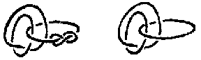
Figure: k055600a
Thus, isotopy of links neglects "small" knots, and therefore its study may be considered as the theory of links modulo the theory of knots. This statement is formulated precisely in the following theorem of Rolfsen [12]: Two isotopic links are enveloping isotopic if their corresponding components are equivalent (as oriented knots). In view of this result the study of isotopy reduces to enveloping isotopy.
Another equivalence relation studied in knot theory is concordance or cobordism. Two locally flat imbeddings $ i _ {0} $ and $ i _ {1} $ of a manifold $ X $ in a manifold $ Y $ are called concordant if there exists a locally flat imbedding
$$ i : X \times [ 0 , 1 ] \rightarrow Y \times [ 0 , 1 ] $$
such that $ i ( x , 0 ) = ( i _ {0} ( x) , 0 ) $, $ i ( x , 1 ) = ( i _ {1} ( x) , 1 ) $ for all $ x \in X $. If $ X $ is the disjoint sum of several copies of a circle and $ Y $ is $ \mathbf R ^ {3} $ or $ S ^ {3} $, then one obtains the definition of concordant links. The connected sum provides the set of concordance classes of knots with an Abelian group structure. The zero of this group is the class containing the trivial knot. A knot concordant to a trivial knot is called a slice knot. The opposite of the class of a knot $ k $ is the class of the knot obtained as follows: change the orientation of $ k $ and take its image under reflection in any plane. About the structure of the group of concordance classes see Cobordism of knots. In order to construct a slice knot one simply takes the trivial $ 2 $- component link, glues on any of its components a tape, knots it in some way, passes it over the initial link and then glues it to the second component. After this it is necessary to remove all the interior points of the tape as well as the boundary points at which the gluing has taken place. As a result a slice knot is obtained (see e.g. Fig. b).
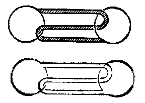
Figure: k055600b
A generalization of this construction leads to the concept of a ribbon knot [1]. There is the conjecture that every slice knot is a ribbon knot. Isotopy of links does not imply their concordance (indeed, every knot is isotopic to the trivial knot, but not every knot is slice). However, isotopic links are concordant if all their corresponding components are pairwise concordant [12].
Other equivalence relations between links have also been studied, e.g. homotopy and $ I $- equivalence (cf. [8]).
The apparatus of knot theory.
The fundamental group $ G ( L) $ of the complementary space $ M ( L) $ is called the group of the link $ L $. It is a most important algebraic invariant of the link. In the case of knots and indecomposable links the exterior $ M ( L) $ is aspherical and therefore its homotopy type determines $ G ( L) $. A link is trivial if and only if its group is free [8]. Two torus knot are equivalent if and only if they have isomorphic groups. However, the assertion that the group determines the type of a link is false already for knots [1]. There are some descriptions of algorithms for presenting groups of links from their diagrams. The most widely known is the Wirtinger presentation. For properties of groups of links see Knot and link groups.
A stronger invariant of links is the group system $ \langle G ( L) ; T _ {1} \dots T _ \mu \rangle $, consisting of the link group $ G ( L) $ and the conjugacy classes of the subgroups $ T _ {i} $ generated by the classes of the meridians and the parallels of the $ i $- th component. The group system of a knot determines the topological type of its complement. A complete algebraic knot invariant is provided by the triple $ ( G , T , m ) $ consisting of the knot group $ G $, the peripheral subgroup (cf. Knot and link groups) $ T \subset G $ and a meridian $ m \in T $: Two knots are equivalent if and only if there is an isomorphism between their groups that preserves the peripheral subgroup and carries a meridian of one to a meridian of the other or to its inverse. It is known how to classify the invariants of knots represented by their groups. One such invariant [11] associated with the knot $ k $ is the free product of the group of a certain winding of the connected sum of the knot $ k $ and the Listing knot $ 4 _ {1} $. In this definition instead of the knot $ 4 _ {1} $ one can take any other knot and so obtain a group which, although altered, is as before a complete invariant.
One can find (cf. [5]) a more natural complete algebraic knot invariant. Let a knot $ k $ be given by its regular projection on a plane, and let all its overpasses be numbered from 1 to $ n $. Suppose further that in some double point the passes numbered $ p , q , r $ meet, as in Fig. c, and let $ \Gamma ( k) $ be the distributive groupoid given by the generators $ a _ {1} \dots a _ {n} $( their number being equal to the number of passes) with the relations $ a _ {p} \circ a _ {q} = a _ {r} $( one for each double point).

Figure: k055600c
One can prove (cf. [5]) that, first, the groupoid $ \Gamma ( k) $ is an invariant of the knot, i.e. does not depend on the choice of the projection, and, secondly, that knots with isomorphic groupoids are equivalent.
The group of the knot, the group system and the groupoid are quite complex algebraic objects and distinguishing them is often not an easy case. In calculations it is convenient to have Abelian invariants of knots and links, with which it is easier to work (e.g. they can be described by commutative algebra) and which at the same time provide enough information. The most important algebraic invariant is the Alexander module, defined as follows. The homology group $ H _ {1} ( M ( L) ) $ of the exterior of a link of multiplicity $ \mu $ is a free Abelian group of rank $ \mu $( this is a consequence of Alexander duality) and therefore the covering mapping $ p : \widetilde{M} ( L) \rightarrow M ( L) $ corresponding to the commutator subgroup of $ G ( L) $ has $ \mathbf Z ^ \mu $ as group of covering transformations. If $ x _ {0} \in M ( L) $ is a basis point and $ \widetilde{X} {} _ {0} = p ^ {-} 1 ( x _ {0} ) $, then the group $ H _ {1} ( \widetilde{M} ( L) , \widetilde{X} {} _ {0} ) $ has the natural structure of a module over $ \Lambda _ \mu = \mathbf Z [ \mathbf Z ^ \mu ] $( the ring of integral Laurent polynomials in $ \mu $ variables), which is called the Alexander module of the link $ L $. In the case $ \mu = 1 $ the module $ H _ {1} ( \widetilde{M} ( L) , \widetilde{X} _ {0} ) $ is isomorphic to the direct sum of $ H _ {1} ( \widetilde{M} ( L) ) $ and $ \Lambda _ {1} $; therefore, in the study of knots one also calls the $ \Lambda _ {1} $- module $ H _ {1} ( \widetilde{M} ( L) ) $ the Alexander module. The matrix giving a presentation of the Alexander module is called the Alexander matrix. To find the Alexander matrix from a presentation of the group $ G ( L) $ one uses the free differential calculus of Fox [1]. The Alexander module gives in a standard manner (cf. Alexander invariants) an ascending chain of ideals of the ring $ \Lambda _ \mu $( called elementary ideals) and a sequence of integral polynomials $ \Delta _ {1} ( t _ {1} \dots t _ \mu ) , \Delta _ {2} ( t _ {1} \dots t _ \mu ) \dots $ defined up to units in $ \Lambda _ \mu $. The first polynomial $ \Delta _ {1} ( t _ {1} \dots t _ \mu ) $ is called the Alexander polynomial. The Alexander module also defines the Steinitz–Fox–Smythe class of ideals [8]. With its help one is able to prove, for example, the non-invertibility of certain knots (a knot $ k \subset S ^ {3} $ is called invertible if there exists an orientation-preserving homeomorphism of $ S ^ {3} $ onto itself transforming $ k $ to $ k $ with the opposite orientation). The invertibility of a knot implies the following property of the Alexander module: There exists a group automorphism $ f : H _ {1} ( \widetilde{M} ( k) ) \rightarrow H _ {1} ( \widetilde{M} ( k) ) $ with $ f ( t a ) = t ^ {-} 1 f ( a) $ for any $ a \in H _ {1} ( \widetilde{M} ( k) ) $.
A link polynomial has the following reciprocity property: For any $ i \geq 1 $ the principal ideals of the ring $ \Lambda _ \mu $ generated by $ \Delta _ {i} ( t _ {1} \dots t _ \mu ) $ and $ \Delta _ {i} ( t _ {1} ^ {-} 1 \dots t _ \mu ^ {-} 1 ) $ coincide. This fact exhibits a basic kind of duality in the homology of the universal Abelian covering of the exterior of the link. The duality not only imposes a restriction on the Alexander module, but also endows it with an additional multiplicative structure. E.g., in the case of a knot one has an invariantly defined non-degenerate Hermitian form
$$ H _ {1} ( \widetilde{M} ( L) ) \times H _ {1} ( \widetilde{M} ( L) ) \rightarrow \ Q ( \Lambda ) / \Lambda , $$
called the Blanchfield form. Here $ \Lambda = \Lambda _ {1} $ and $ Q ( \Lambda ) $ is the field of fractions of $ \Lambda $. For the definition and analogous properties of this form for links see [8]. Closely connected with the Blanchfield form is the Milnor form, taking values in $ \mathbf Q $( cf. [6]). The Seifert matrix corresponding to any Seifert surface of a knot determines the Alexander module and the Blanchfield and Milnor forms on it [13]. If $ k _ {1} $ and $ k _ {2} $ are two knots, then the following properties are equivalent: 1) $ k _ {1} $ and $ k _ {2} $ have isomorphic Blanchfield forms; 2) $ k _ {1} $ and $ k _ {2} $ have isomorphic Milnor forms; and 3) the Seifert matrices of $ k _ {1} $ and $ k _ {2} $ are $ S $- equivalent (cf. [6]).
Every epimorphism $ \phi $ of the group $ G ( L) $ of a link onto an arbitrary group $ H $ defines a regular covering of the exterior $ M ( L) $ with $ H $ as group of covering transformations. If $ H $ is a finite group, then by glueing in a corresponding manner semi-tori to the boundary of the covering, one obtains a manifold $ \Sigma _ \phi ( L) $ and a mapping $ \Sigma _ \phi ( L) \rightarrow S ^ {3} $ which is a ramified covering with ramification over $ L $. The group $ H $ acts on $ \Sigma _ \phi ( L) $. Therefore $ B _ \phi = H _ {1} ( \Sigma _ \phi ( L) ) $ is a $ \mathbf Z [ H] $- module. Moreover, since $ \Sigma _ \phi ( L) $ is a closed oriented $ 3 $- dimensional manifold, it defines a form of link coefficients
$$ \{ , \} : \ \mathop{\rm Tors} _ {\mathbf Z} B _ \phi \times \mathop{\rm Tors} _ {\mathbf Z} B _ \phi \rightarrow \mathbf Q / \mathbf Z . $$
Thus, to every representation $ \phi : G ( L) \rightarrow H $ on a finite group $ H $ corresponds a $ \mathbf Z [ H] $- module $ B _ \phi $ and a pairing $ \{ , \} $.
The representation of groups of links in cyclic and metacyclic groups has been thoroughly studied. The group of an oriented link admits a canonical representation on a cyclic group $ \mathbf Z _ {n} $( the class of a loop $ \alpha $ consists of the residue modulo $ n $ of the link coefficient of $ \alpha $ with $ L $). This representation corresponds to a ramified covering $ \Sigma _ \phi ( L) \rightarrow S ^ {3} $, called an $ n $- sheeted cyclic ramified covering of the link $ L $. It corresponds to an invariant $ ( B _ \phi , \{ , \} ) $ which is often used to distinguish knots. It is expressed by the Seifert matrix and hence by the Alexander module with the Blanchfield pairing.
A very effective invariant of knots and links is the Conway polynomial. Its calculation is much simpler than that of the Alexander polynomial (it does not require to find the Alexander matrix, to compute its determinant, etc.). In order to calculate the Conway polynomial one does not need its definition but only the following three properties: 1) the Conway polynomial $ \nabla _ {L} ( z) $ is an invariant of the enveloping isotopy type of an oriented link $ L $; 2) if $ L $ is the trivial knot, then $ \nabla _ {L} ( z) = 1 $; and 3) if three links $ L _ {+} $, $ L _ {-} $ and $ L _ {0} $ have diagrams which coincide apart from the parts shown in Fig. d, then
$$ \nabla _ {L _ {+} } ( z) - \nabla _ {L _ {-} } ( z) = \ z \nabla _ {L _ {0} } ( z) . $$
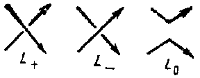
Figure: k055600d
These properties imply, e.g., that the Conway polynomial of a split link is equal to zero. Thanks to property 3) one can follow the changes of the Conway polynomial when varying diagrams in separate double points; it is clear that after a finite number of such modifications the link becomes trivial and at that point the calculation is complete. A theory which facilitates finding the Conway polynomial has been developed in [14]. For knots the Conway and Alexander polynomials determine each other uniquely. E.g., from knowledge of the Conway polynomial the Alexander polynomial $ \Delta ( t) $ is defined by the equation $ \Delta ( t ^ {2} ) = t ^ {2n} \nabla _ {L} ( t - t ^ {-} 1 ) $.
Classification of knots and links.
Above, complete algebraic knot invariants with the help of which the problem of distinguishing different knots is reduced to algebra have been mentioned. An algorithm for calculating the genus of a knot was constructed by H. Haken, but it is not very practical. For certain classes, e.g. for alternating knots and links, there is a simple algorithm (cf. also Neuwirth knot).
All knots having a diagram with at most 11 double points have been enumerated; likewise for all links having fewer than 11 crossings (cf. [17]). However, it has not been proved that among the knots on this list having 11 crossing there are no repetitions. For a table of simple knots having nine or fewer crossings cf. Knot table.
The torus knots have been completely classified, as have the knots with two bridges (cf. [16]).
In connection with the development of the topology of manifolds there is the study of multi-dimensional knots and links; multi-dimensional knot theory has been developed better in several respects than the classical theory. Thus, the solution of the problem of classifying multi-dimensional knots by means of cobordism (cf. Cobordism of knots) is complete, a description of the enveloping isotopy classes of multi-dimensional knots in terms of stable homotopy has been obtained [15] and the most important forms of multi-dimensional knots have been distinguished by algebraic invariants [6]. Moreover, homological invariants of multi-dimensional knots have been found which determine their type up to a finite number of possibilities.
Applications of knot theory.
The merit of knot theory for the study of $ 3 $- dimensional manifolds consists, first of all, in that every closed oriented $ 3 $- dimensional manifold can be represented as a covering of the sphere $ S ^ {3} $, ramified over a certain link (Alexander's theorem). Furthermore (cf. [16]), every oriented connected $ 3 $- dimensional manifold of genus 1 (i.e. a lens space) is homeomorphic to a two-sheeted ramified covering of a certain link with two bridges, and links with two bridges are equivalent if only if their two-sheeted ramified coverings are isomorphic. This fact is useful in the description of $ 3 $- dimensional manifolds as well as in the classification of knots.
Every oriented connected $ 3 $- dimensional manifold of genus two is homeomorphic to a two-sheeted ramified covering of a certain link with three bridges; an example of non-equivalent knots with three bridges having homeomorphic two-sheeted ramified coverings has been constructed (cf. [4]).
Another important consequence furnished by knot theory in the study of $ 3 $- dimensional manifolds is the calculation of framed links by R.C. Kirby [3]. A framed link is a finite set $ L $ of non-intersecting smooth imbeddings of circles $ l _ {1} \dots l _ \mu \subset S ^ {3} $( knotted or not), each taken a certain number $ n _ {i} $. A framed link $ L $ defines a $ 4 $- dimensional manifold $ M _ {L} $, obtained by glueing on a $ 4 $- dimensional sphere a handle of index two, where the glueing mapping $ f _ {i} : S ^ {1} \times D ^ {2} \rightarrow S ^ {3} $ of the $ i $- th handle has the properties: 1) $ f _ {i} ( S ^ {1} \times 0 ) = l _ {i} $; and 2) for any $ x \in D ^ {2} \setminus 0 $ the linking coefficient of the curve $ f _ {i} ( S ^ {1} \times \{ x \} ) $ with $ l _ {i} $ is $ n _ {i} $. The boundary $ W _ {L} = \partial M _ {L} $ is a closed oriented $ 3 $- dimensional manifold. It turns out that, first, every closed oriented $ 3 $- dimensional manifold is homeomorphic to $ W _ {L} $ for a certain framed link $ L $ and, secondly, $ W _ {L _ {1} } $ and $ W _ {L _ {2} } $ are homeomorphic if and only if the framed link $ L _ {1} $ can be obtained from $ L _ {2} $ by the transformations $ {\mathcal O} _ {1} $ and $ {\mathcal O} _ {2} $ described below or by their inverses. The transformation $ {\mathcal O} _ {1} $ consists of supplementing a framed link by an unknotted circle, separating the remaining components of the imbedded $ 2 $- sphere, taken with $ + 1 $ or $ - 1 $. The transformation $ {\mathcal O} _ {2} $ effects the "composition" of two components $ l _ {i} $ and $ l _ {j} $ in the following manner: Let $ \widetilde{l} _ {i} $ be a curve on the boundary of a small tubular neighbourhood of $ l _ {i} $ in $ S ^ {3} $, isotopic to $ l _ {i} $ in this tubular neighbourhood and having linking coefficient $ n _ {i} $ with $ l _ {i} $. Replace the component $ l _ {i} $ by the circle $ l _ {j} ^ \prime = l _ {j} \# _ {b} \widetilde{l} _ {i} $, where $ b $ is a certain ribbon joining $ l _ {j} $ and $ \widetilde{l} _ {i} $ but not touching the remaining parts of the link $ L $, and so obtain a new link $ L ^ \prime $ if the new component $ l _ {j} ^ \prime $ is assigned the number $ n _ {j} ^ \prime = n _ {i} + n _ {j} \pm 2a _ {ij} $. Here $ a _ {ij} $ is the linking coefficient of $ l _ {i} $ and $ l _ {j} $( oriented in any way) and the sign $ + $ or $ - $ is chosen depending only on the way the orientation of the ribbon is fixed. E.g., for the framed link shown in Fig. ethe manifold $ W _ {L} $ is the corresponding lens space $ L ( n , 1 ) $ in case a), the lens space $ L ( p q - 1 , p ) = L ( p q - 1 , q ) $ in case b) and the dodecahedral space in cases c) and d). a) b) c) d)
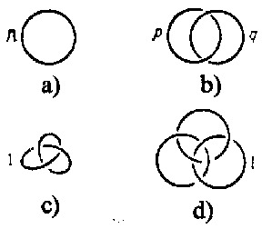
Figure: k055600e
Apart from these and many other uses of knot theory in topology, its applications include also the study of singularities of plane algebraic curves, and in the multi-dimensional case — the study of isolated singularities of complex hypersurfaces [2], smooth structures on spheres, and the construction of dynamical systems and stratifications. There are attempts to apply knot theory in symbolic dynamics [18] and in the mathematical theory of turbulence [19].
Historical information.
Apparently C.F. Gauss was the first to consider knots as mathematical objects. He reckoned that the analysis of knotting and linking was one of the basic objects of "geometry situs" . Gauss himself wrote little on knots and links (cf. Linking coefficient), but his student J.B. Listing devoted a considerable part of his monograph [7] to knots.
At the end of the 19th century, tables of simple knots having at most ten crossing were composed by the efforts of P.G. Tait and C. Little, as well as tables of alternating simple knots with at most 11 crossings. The problem of tabulating knots has two aspects: first one has to convince oneself that the list represented is complete and secondly one must show that all the knots enumerated are really different. At that time, while the solution of the first problem only required combinatorial reasoning (though cumbersome enough), for an answer to the second question invariants of algebraic topology were necessary. Such invariants did not exist in the 19th century, therefore the non-equivalence of the listed knots in a table was justified empirically. Subsequent analysis detected several errors in the tables of the 19th century.
In 1906 H. Tietze was the first to apply the fundamental group for the proof of the non-triviality of a knot. In 1927 J.W. Alexander and G.B. Briggs, using the torsion coefficients of the homology of two- and three-sheeted ramified cyclic coverings, distinguished all tabulated knots with 8 crossings and all knots, with the exception of three pairs, with 9 crossings. In 1928 there appeared the Alexander polynomial, but its help still did not remove all doubts about the distinctness of the 84 knots having at most 9 crossings. This last step was taken by K. Reidemeister, by a consideration of the linking coefficients in a dihedral ramified covering.
A presentation of the current state of knot theory is given in the list of problems [10]; in it comments and bibliographical references can also be found. Similar bibliographies on knot theory can be found in [1], [8], [9].
References
| [1] | R.H. Crowell, R.H. Fox, "Introduction to knot theory" , Ginn (1963) MR0146828 Zbl 0126.39105 |
| [2] | J. Milnor, "Singular points of complex hypersurfaces" , Princeton Univ. Press (1968) MR0239612 Zbl 0184.48405 |
| [3] | R. Mandelbaum, "Four-dimensional topology" Bull. Amer. Math. Soc. , 2 (1980) pp. 1–159 MR0551752 Zbl 0476.57005 |
| [4] | O.Ya. Viro, "Linkings, two-sheeted branched coverings and braids" Math. USSR Sb. , 16 (1972) pp. 223–236 Mat. Sb. , 87 (1972) pp. 216–228 Zbl 0248.55002 |
| [5] | S.V. Matveev, "Distributive groupoids in knot theory" Math. USSR Sb. , 47 (1984) pp. 73–83 Mat. Sb. , 119 (1982) pp. 78–88 MR0672410 Zbl 0523.57006 |
| [6] | M.Sh. Farber, "The classification of simple knots" Russian Math. Surveys , 38 : 5 (1983) pp. 63–117 Uspekhi Mat. Nauk , 38 : 5 (1983) pp. 59–106 MR718824 Zbl 0546.57006 |
| [7] | I.B. Listing, "Vorstudien zur Topologie" , Göttingen (1848) |
| [8] | J.A. Hillman, "Alexander ideals of links" , Springer (1981) MR0653808 Zbl 0491.57001 |
| [9] | C.McA. Gordon, "Some aspects of clasical knot theory" , Knot theory. Proc. Sem. Plans-sur-Bex, 1977 , Lect. notes in math. , 685 , Springer (1978) pp. 1–60 |
| [10] | R.C. Kirby, "Problems in low dimensional manifold theory" , Algebraic geometry and geometric topology , Proc. Symp. Pure Math. , 32 , Amer. Math. Soc. (1978) pp. 273–312 MR0520548 Zbl 0394.57002 |
| [11] | J. Simon, "An algebraic classification of knots in  " Ann. of Math. , 97 (1973) pp. 1–13 MR0310861 Zbl 0256.55003 " Ann. of Math. , 97 (1973) pp. 1–13 MR0310861 Zbl 0256.55003 |
| [12] | D. Rolfsen, "Isotopy of links in codimension two" J. Indian Math. Soc. , 36 (1972) pp. 263–278 MR0341497 Zbl 0276.57005 |
| [13] | J. Levine, "Knot modules I" Trans. Amer. Math. Soc. , 229 (1977) pp. 1–50 MR0461518 Zbl 0653.57012 |
| [14] | C.A. Giller, "A family of links and the Conway calculus" Trans. Amer. Math. Soc. , 270 (1982) pp. 75–109 MR0642331 Zbl 0492.57002 |
| [15] | M.Sh. Farber, "Isotopy types of knots of codimension two" Trans. Amer. Math. Soc. , 261 (1980) pp. 185–209 MR0576871 Zbl 0513.57007 |
| [16] | H. Schubert, "Knoten mit zwei Brücken" Math. Z. , 65 (1956) pp. 133–170 MR0082104 Zbl 0071.39002 |
| [17] | J.H. Conway, "An enumeration of knots and links, and some of their algebraic properties" , Computational problems in abstract algebra , Pergamon (1970) pp. 329–358 MR0258014 Zbl 0202.54703 |
| [18] | J.M. Franks, "Knots, links and symbolic dynamics" Ann. of Math. , 113 (1981) pp. 529–552 MR0621015 Zbl 0469.58013 |
| [19] | J.S. Birman, R.F. Williams, "Knotted periodic orbits in dynamical systems. I Lorenz's equations" Topology , 22 (1983) pp. 47–82 MR0682059 MR0718132 |
Comments
A remarkable breakthrough in knot theory has taken place recently. It started in 1984 with the discovery of a new polynomial invariant (in two variables), the Jones polynomial, that can distinguish between some knots that have the same Alexander polynomial, [a4], [a5]. The Jones polynomial was soon followed by other new polynomial invariants, first the so-called HOMFLY polynomial, [a9], and also, independently, [a11], and soon after several others.
These polynomials "come from" fields in mathematics previously thought largely unrelated to knot theory: von Neumann algebras (the Jones polynomial), exactly-solvable models in lattice statistical mechanics, quantum field theory. Thus, e.g., the original Jones polynomial "belongs to" a Potts model and both the HOMFLY polynomial and the Kauffman polynomial have specializations belonging to other "Yang–Baxter modelYang–Baxter models" . A central role in all this is played by the Yang–Baxter equation.
A selection of recent literature on these matters is [a4]–[a12].
Like the Conway polynomial (cf. the main article above), the Jones polynomial can be described in terms of certain "moves" for changing knots. Apparently these moves are the same which occur as during replication DNA unknots and knots itself, [a13]. For other aspects of DNA involving the linking number, total twist and writhing number of a knot cf. [a14].
References
| [a1] | D. Rolfsen, "Knots and links" , Publish or Perish (1976) MR0515288 Zbl 0339.55004 |
| [a2] | L.H. Kauffman, "On knots" , Princeton Univ. Press (1987) pp. Sect. 18; Appendix MR0907872 Zbl 0627.57002 |
| [a3] | J.S. Birman, "Braids, links and mapping class groups" , Princeton Univ. Press (1975) MR0425944 Zbl 0305.57013 |
| [a4] | V.F.R. Jones, "A polynomial invariant for knots and links via von Neumann algebras" Bull. Amer. Math. Soc. , 12 (1985) pp. 103–111 |
| [a5] | V.F.R. Jones, "Hecke algebra representations of braid groups and link polynomials" Ann. of Math. , 126 (1987) pp. 335–388 MR0908150 Zbl 0631.57005 |
| [a6] | L.H. Kauffman, "State models for link polynomials" , Reprint , M/88/46 , IHES (1988) MR1071412 Zbl 0711.57003 |
| [a7] | V.G. Turaev, "The Yang–Baxter equation and invariants of links" Invent. Math. , 92 (1988) pp. 527–553 MR0939474 Zbl 0648.57003 |
| [a8] | E. Witten, "Quantum field theory and the Jones polynomial" , IAMP congress, Swansea, July 1988 MR1338609 MR1062429 MR0990772 Zbl 0818.57014 Zbl 0726.57010 Zbl 0667.57005 |
| [a9] | P. Freyd, D. Yetter, J. Hoste, W.R.R. Lickorish, K. Millett, A. Ocneanu, "A new polynomial invariant of knots and links" Bull. Amer. Math. Soc. , 12 (1985) pp. 239–246 MR0776477 Zbl 0572.57002 |
| [a10] | L. Kauffman, "State models and the Jones polynomial" Topology , 26 (1987) pp. 395–407 MR0899057 Zbl 0622.57004 |
| [a11] | J.H. Przytycki, P. Traczyk, "Invariants of links of Conway type" Kobe J. Math. , 4 (1987) pp. 115–139 MR0945888 Zbl 0655.57002 |
| [a12] | Y. Akutsu, M. Wadati, "Knots, links, braids and exactly solvable models in statistical mechanics" Comm. Math. Phys. , 117 (1988) pp. 243–259 MR0947003 Zbl 0651.57005 |
| [a13] | G. Kolata, "Solving knotty problems in math and biology" Science , 231 (1986) pp. 1506–1508 MR0832616 Zbl 1226.57001 |
| [a14] | W.F. Pohl, "DNA and differential geometry" Math. Intelligencer , 3 (1980) pp. 20–27 MR0617886 Zbl 0447.92013 |
Knot theory. Encyclopedia of Mathematics. URL: http://encyclopediaofmath.org/index.php?title=Knot_theory&oldid=15522