Difference between revisions of "Integral calculus"
(Importing text file) |
Ulf Rehmann (talk | contribs) m (tex encoded by computer) |
||
| Line 1: | Line 1: | ||
| + | <!-- | ||
| + | i0513601.png | ||
| + | $#A+1 = 154 n = 0 | ||
| + | $#C+1 = 154 : ~/encyclopedia/old_files/data/I051/I.0501360 Integral calculus | ||
| + | Automatically converted into TeX, above some diagnostics. | ||
| + | Please remove this comment and the {{TEX|auto}} line below, | ||
| + | if TeX found to be correct. | ||
| + | --> | ||
| + | |||
| + | {{TEX|auto}} | ||
| + | {{TEX|done}} | ||
| + | |||
The branch of mathematics in which the notion of an [[Integral|integral]], its properties and methods of calculation are studied. Integral calculus is intimately related to [[Differential calculus|differential calculus]], and together with it constitutes the foundation of mathematical analysis. The origin of integral calculus goes back to the early period of development of mathematics and it is related to the method of exhaustion developed by the mathematicians of Ancient Greece (cf. [[Exhaustion, method of|Exhaustion, method of]]). This method arose in the solution of problems on calculating areas of plane figures and surfaces, volumes of solid bodies, and in the solution of certain problems in statistics and hydrodynamics. It is based on the approximation of the objects under consideration by stepped figures or bodies, composed of simplest planar figures or special bodies (rectangles, parallelopipeds, cylinders, etc.). In this sense, the method of exhaustion can be regarded as an early method of integration. The greatest development of the method of exhaustion in the early period was obtained in the works of Eudoxus (4th century B.C.) and especially Archimedes (3rd century B.C.). Its subsequent application and perfection is associated with the names of several scholars of the 15th–17th centuries. | The branch of mathematics in which the notion of an [[Integral|integral]], its properties and methods of calculation are studied. Integral calculus is intimately related to [[Differential calculus|differential calculus]], and together with it constitutes the foundation of mathematical analysis. The origin of integral calculus goes back to the early period of development of mathematics and it is related to the method of exhaustion developed by the mathematicians of Ancient Greece (cf. [[Exhaustion, method of|Exhaustion, method of]]). This method arose in the solution of problems on calculating areas of plane figures and surfaces, volumes of solid bodies, and in the solution of certain problems in statistics and hydrodynamics. It is based on the approximation of the objects under consideration by stepped figures or bodies, composed of simplest planar figures or special bodies (rectangles, parallelopipeds, cylinders, etc.). In this sense, the method of exhaustion can be regarded as an early method of integration. The greatest development of the method of exhaustion in the early period was obtained in the works of Eudoxus (4th century B.C.) and especially Archimedes (3rd century B.C.). Its subsequent application and perfection is associated with the names of several scholars of the 15th–17th centuries. | ||
| Line 5: | Line 17: | ||
By means of integral calculus it became possible to solve by a unified method many theoretical and applied problems, both new ones which earlier had not been amenable to solution, and old ones that had previously required special artificial techniques. The basic notions of integral calculus are two closely related notions of the integral, namely the indefinite and the definite integral. | By means of integral calculus it became possible to solve by a unified method many theoretical and applied problems, both new ones which earlier had not been amenable to solution, and old ones that had previously required special artificial techniques. The basic notions of integral calculus are two closely related notions of the integral, namely the indefinite and the definite integral. | ||
| − | The indefinite integral of a given real-valued function on an interval on the real axis is defined as the collection of all its primitives on that interval, that is, functions whose derivatives are the given function. The indefinite integral of a function | + | The indefinite integral of a given real-valued function on an interval on the real axis is defined as the collection of all its primitives on that interval, that is, functions whose derivatives are the given function. The indefinite integral of a function $ f $ |
| + | is denoted by $ \int f ( x) d x $. | ||
| + | If $ F $ | ||
| + | is some primitive of $ f $, | ||
| + | then any other primitive of it has the form $ F + C $, | ||
| + | where $ C $ | ||
| + | is an arbitrary constant; one therefore writes | ||
| − | + | $$ | |
| + | \int\limits f ( x) d x = F ( x) + C . | ||
| + | $$ | ||
The operation of finding an indefinite integral is called integration. Integration is the operation inverse to that of differentiation: | The operation of finding an indefinite integral is called integration. Integration is the operation inverse to that of differentiation: | ||
| − | + | $$ | |
| + | \int\limits F ^ { \prime } ( x) d x = F ( x) + C ,\ \ | ||
| + | d \int\limits f ( x) d x = f ( x) d x . | ||
| + | $$ | ||
The operation of integration is linear: If on some interval the indefinite integrals | The operation of integration is linear: If on some interval the indefinite integrals | ||
| − | + | $$ | |
| + | \int\limits f _ {1} ( x) d x \ \textrm{ and } \ \int\limits f _ {2} ( x) d x | ||
| + | $$ | ||
| − | exist, then for any real numbers | + | exist, then for any real numbers $ \lambda _ {1} $ |
| + | and $ \lambda _ {2} $, | ||
| + | the following integral exists on this interval: | ||
| − | + | $$ | |
| + | \int\limits [ \lambda _ {1} f _ {1} ( x) + \lambda _ {2} f _ {2} ( x) ] \ | ||
| + | d x | ||
| + | $$ | ||
and equals | and equals | ||
| − | + | $$ | |
| + | \lambda _ {1} \int\limits f _ {1} ( x) d x + \lambda _ {2} \int\limits f _ {2} ( x) d x . | ||
| + | $$ | ||
| − | For indefinite integrals, the formula of [[Integration by parts|integration by parts]] holds: If two functions | + | For indefinite integrals, the formula of [[Integration by parts|integration by parts]] holds: If two functions $ u $ |
| + | and $ v $ | ||
| + | are differentiable on some interval and if the integral $ \int v d u $ | ||
| + | exists, then so does the integral $ \int u d v $, | ||
| + | and the following formula holds: | ||
| − | + | $$ | |
| + | \int\limits u d v = u v - \int\limits v d u . | ||
| + | $$ | ||
| − | The formula for change of variables holds: If for two functions | + | The formula for change of variables holds: If for two functions $ f $ |
| + | and $ \phi $ | ||
| + | defined on certain intervals, the composite function $ f \circ \phi $ | ||
| + | makes sense and the function $ \phi $ | ||
| + | is differentiable, then the integral | ||
| − | + | $$ | |
| + | \int\limits f [ \phi ( t) ] \phi ^ \prime ( t) d t | ||
| + | $$ | ||
exists and equals (see [[Integration by substitution|Integration by substitution]]) | exists and equals (see [[Integration by substitution|Integration by substitution]]) | ||
| − | + | $$ | |
| + | \int\limits f ( x) d x . | ||
| + | $$ | ||
A function that is continuous on some bounded interval has a primitive on it and hence an indefinite integral exists for it. The problem of actually finding the indefinite integral of a specified function is complicated by the fact that the indefinite integral of an elementary function is not an elementary function, in general. Many classes of functions are known for which it proves possible to express their indefinite integrals in terms of elementary functions. The simplest examples of these are integrals that are obtained from a table of derivatives of the basic elementary functions (see [[Differential calculus|Differential calculus]]): | A function that is continuous on some bounded interval has a primitive on it and hence an indefinite integral exists for it. The problem of actually finding the indefinite integral of a specified function is complicated by the fact that the indefinite integral of an elementary function is not an elementary function, in general. Many classes of functions are known for which it proves possible to express their indefinite integrals in terms of elementary functions. The simplest examples of these are integrals that are obtained from a table of derivatives of the basic elementary functions (see [[Differential calculus|Differential calculus]]): | ||
| − | 1) | + | 1) $ \int x ^ \alpha d x = |
| + | \frac{x ^ {\alpha + 1 } }{\alpha + 1 } | ||
| + | + C $, | ||
| + | $ \alpha \neq - 1 $; | ||
| − | 2) | + | 2) $ \int |
| + | \frac{dx}{x} | ||
| + | = \mathop{\rm ln} | x | + C $; | ||
| − | 3) | + | 3) $ \int a ^ {x} d x = |
| + | \frac{a ^ {x} }{ \mathop{\rm ln} a } | ||
| + | + C $, | ||
| + | $ a > 0 $, | ||
| + | $ a \neq 1 $; | ||
| + | in particular, $ \int e ^ {x} d x = e ^ {x} + C $; | ||
| − | 4) | + | 4) $ \int \sin x d x = - \cos x + C $; |
| − | 5) | + | 5) $ \int \cos x d x = \sin x + C $; |
| − | 6) | + | 6) $ \int |
| + | \frac{dx}{\cos ^ {2} x } | ||
| + | = \mathop{\rm tan} x + C $; | ||
| − | 7) | + | 7) $ \int |
| + | \frac{dx}{\sin ^ {2} x } | ||
| + | = - \mathop{\rm cotan} x + C $; | ||
| − | 8) | + | 8) $ \int \sinh x d x = \cosh x + C $; |
| − | 9) | + | 9) $ \int \cosh x d x = \sinh x + C $; |
| − | 10) | + | 10) $ \int |
| + | \frac{dx}{\cosh ^ {2} x } | ||
| + | = \mathop{\rm tanh} x + C $; | ||
| − | 11) | + | 11) $ \int |
| + | \frac{dx}{\sinh ^ {2} x } | ||
| + | = - \mathop{\rm cotanh} x + C $; | ||
| − | 12) | + | 12) $ \int |
| + | \frac{dx}{x ^ {2} + a ^ {2} } | ||
| + | = | ||
| + | \frac{1}{a} | ||
| + | \mathop{\rm arctan} | ||
| + | \frac{x}{a} | ||
| + | + C = - | ||
| + | \frac{1}{a} | ||
| + | \mathop{\rm arccotan} | ||
| + | \frac{x}{a} | ||
| + | + C ^ \prime $; | ||
| − | 13) | + | 13) $ \int |
| + | \frac{dx}{x ^ {2} - a ^ {2} } | ||
| + | = | ||
| + | \frac{1}{2a} | ||
| + | \mathop{\rm ln} \left | x- | ||
| + | \frac{a}{x+} | ||
| + | a \right | + C $; | ||
| − | 14) | + | 14) $ \int |
| + | \frac{dx}{\sqrt {a ^ {2} - x ^ {2} } } | ||
| + | = \mathop{\rm arcsin} | ||
| + | \frac{x}{a} | ||
| + | + C = - \mathop{\rm arccos} | ||
| + | \frac{x}{a} | ||
| + | + C ^ \prime $, | ||
| + | $ | x | < | a | $; | ||
| − | 15) | + | 15) $ \int |
| + | \frac{dx}{\sqrt {x ^ {2} \pm a ^ {2} } } | ||
| + | = \mathop{\rm ln} | x + \sqrt {x ^ {2} \pm a ^ {2} } | + C $( | ||
| + | when $ x ^ {2} - a ^ {2} $ | ||
| + | is under the square root, it is assumed that $ | x | > | a | $). | ||
If the denominator of the integrand vanishes at some point, then these formulas are valid only for those intervals inside which the denominator does not vanish (see formulas 1, 2, 6, 7, 11, 13, 15). | If the denominator of the integrand vanishes at some point, then these formulas are valid only for those intervals inside which the denominator does not vanish (see formulas 1, 2, 6, 7, 11, 13, 15). | ||
| Line 73: | Line 164: | ||
The indefinite integral of a rational function over any interval on which the denominator does not vanish is a composition of rational functions, arctangents and natural logarithms. Finding the algebraic part of the indefinite integral of a rational function can be achieved by the [[Ostrogradski method|Ostrogradski method]]. Integrals of the following types can be reduced by means of substitution and integration by parts to integration of rational functions: | The indefinite integral of a rational function over any interval on which the denominator does not vanish is a composition of rational functions, arctangents and natural logarithms. Finding the algebraic part of the indefinite integral of a rational function can be achieved by the [[Ostrogradski method|Ostrogradski method]]. Integrals of the following types can be reduced by means of substitution and integration by parts to integration of rational functions: | ||
| − | + | $$ | |
| + | \int\limits R | ||
| + | \left [ | ||
| + | x , \left ( | ||
| + | |||
| + | \frac{a x + b }{c x + b } | ||
| + | |||
| + | \right ) ^ {r _ {1} } \dots | ||
| + | \left ( | ||
| + | |||
| + | \frac{a x + b }{c x + b } | ||
| + | |||
| + | \right ) ^ {r _ {m} } | ||
| + | \right ] d x , | ||
| + | $$ | ||
| − | where | + | where $ r _ {1} \dots r _ {m} $ |
| + | are rational numbers; integrals of the form | ||
| − | + | $$ | |
| + | \int\limits R ( x , \sqrt {a x ^ {2} + b x + c } ) d x | ||
| + | $$ | ||
(see [[Euler substitutions|Euler substitutions]]); certain cases of integrals of differential binomials (cf. [[Differential binomial|Differential binomial]]; [[Chebyshev theorem on the integration of binomial differentials|Chebyshev theorem on the integration of binomial differentials]]); integrals of the form | (see [[Euler substitutions|Euler substitutions]]); certain cases of integrals of differential binomials (cf. [[Differential binomial|Differential binomial]]; [[Chebyshev theorem on the integration of binomial differentials|Chebyshev theorem on the integration of binomial differentials]]); integrals of the form | ||
| − | + | $$ | |
| + | \int\limits R ( \sin x , \cos x ) d x ,\ \ | ||
| + | \int\limits R ( \sinh x , \cosh x ) d x | ||
| + | $$ | ||
| − | (where | + | (where $ R ( y _ {1} \dots y _ {n} ) $ |
| + | are rational functions); the integrals | ||
| − | + | $$ | |
| + | \int\limits e ^ {\alpha x } \cos \beta x \ | ||
| + | d x ,\ \int\limits e ^ {\alpha x } \sin \beta x d x , | ||
| + | $$ | ||
| − | + | $$ | |
| + | \int\limits x ^ {n} \cos \alpha x d x ,\ \int\limits x ^ {n} \sin \alpha x d x , | ||
| + | $$ | ||
| − | + | $$ | |
| + | \int\limits x ^ {n} \mathop{\rm arcsin} x d x ,\ \int\limits | ||
| + | x ^ {n} \mathop{\rm arccos} x d x , | ||
| + | $$ | ||
| − | + | $$ | |
| + | \int\limits x ^ {n} \mathop{\rm arctan} x d x ,\ \int\limits x ^ {n} | ||
| + | \mathop{\rm arccotan} x d x ,\ n = 0 , 1 \dots | ||
| + | $$ | ||
and many others. In contrast, for example, the integrals | and many others. In contrast, for example, the integrals | ||
| − | + | $$ | |
| + | \int\limits | ||
| + | \frac{e ^ {x} }{x ^ {n} } | ||
| + | d x ,\ \int\limits | ||
| + | |||
| + | \frac{\sin x }{x ^ {n} } | ||
| + | d x ,\ \int\limits | ||
| + | |||
| + | \frac{\cos x }{x ^ {n} } | ||
| + | d x ,\ n = 1 , 2 \dots | ||
| + | $$ | ||
cannot be expressed in terms of elementary functions. | cannot be expressed in terms of elementary functions. | ||
| Line 101: | Line 234: | ||
The definite integral | The definite integral | ||
| − | + | $$ | |
| + | \int\limits _ { a } ^ { b } f ( x) d x | ||
| + | $$ | ||
| − | of a function | + | of a function $ f $ |
| + | defined on an interval $ [ a , b ] $ | ||
| + | is the limit of integral sums of a specific type (see [[Cauchy integral|Cauchy integral]]; [[Riemann integral|Riemann integral]]; [[Lebesgue integral|Lebesgue integral]]; [[Kolmogorov integral|Kolmogorov integral]]; [[Stieltjes integral|Stieltjes integral]]; etc.). If this limit exists, $ f $ | ||
| + | is said to be Cauchy, Riemann, Lebesgue, etc. integrable. | ||
| − | The geometrical meaning of the integral is tied up with the notion of area: If the function | + | The geometrical meaning of the integral is tied up with the notion of area: If the function $ f \geq 0 $ |
| + | is continuous on the interval $ [ a , b ] $, | ||
| + | then the value of the integral | ||
| − | + | $$ | |
| + | \int\limits _ { a } ^ { b } f ( x) d x | ||
| + | $$ | ||
| − | is equal to the area of the curvilinear trapezium formed by the graph of the function, that is, the set whose boundary consists of the graph of | + | is equal to the area of the curvilinear trapezium formed by the graph of the function, that is, the set whose boundary consists of the graph of $ f $, |
| + | the segment $ [ a , b ] $ | ||
| + | and the two segments on the lines $ x = a $ | ||
| + | and $ x = b $ | ||
| + | making the figure closed, which may degenerate to points (cf. Fig.). | ||
<img style="border:1px solid;" src="https://www.encyclopediaofmath.org/legacyimages/common_img/i051360a.gif" /> | <img style="border:1px solid;" src="https://www.encyclopediaofmath.org/legacyimages/common_img/i051360a.gif" /> | ||
| Line 117: | Line 263: | ||
The calculation of many quantities encountered in practice reduces to the problem of calculating the limit of integral sums; in other words, finding a definite integral; for example, areas of figures and surfaces, volumes of bodies, work done by force, the coordinates of the centre of gravity, the values of the moments of inertia of various bodies, etc. | The calculation of many quantities encountered in practice reduces to the problem of calculating the limit of integral sums; in other words, finding a definite integral; for example, areas of figures and surfaces, volumes of bodies, work done by force, the coordinates of the centre of gravity, the values of the moments of inertia of various bodies, etc. | ||
| − | The definite integral is linear: If two functions | + | The definite integral is linear: If two functions $ f _ {1} $ |
| + | and $ f _ {2} $ | ||
| + | are integrable on an interval $ [ a , b ] $, | ||
| + | then for any real numbers $ \lambda _ {1} $ | ||
| + | and $ \lambda _ {2} $ | ||
| + | the function | ||
| − | + | $$ | |
| + | \lambda _ {1} f _ {1} + \lambda _ {2} f _ {2} $$ | ||
is also integrable on this interval and | is also integrable on this interval and | ||
| − | + | $$ | |
| + | \int\limits _ { a } ^ { b } | ||
| + | [ \lambda _ {1} f _ {1} ( x) + \lambda _ {2} f _ {2} ( x) ] d x = \ | ||
| + | \lambda _ {1} \int\limits _ { a } ^ { b } | ||
| + | f _ {1} ( x) d x + \lambda _ {2} \int\limits _ { a } ^ { b } f _ {2} ( x) d x . | ||
| + | $$ | ||
| − | Integration of a function over an interval has the property of monotonicity: If the function | + | Integration of a function over an interval has the property of monotonicity: If the function $ f $ |
| + | is integrable on the interval $ [ a , b ] $ | ||
| + | and if $ [ c , d ] \subset [ a , b ] $, | ||
| + | then $ f $ | ||
| + | is integrable on $ [ c , d ] $ | ||
| + | as well. The integral is also additive with respect to the intervals over which the integration is carried out: If $ a < c < b $ | ||
| + | and the function $ f $ | ||
| + | is integrable on the intervals $ [ a , c ] $ | ||
| + | and $ [ c , b ] $, | ||
| + | then it is integrable on $ [ a , b ] $, | ||
| + | and | ||
| − | + | $$ | |
| + | \int\limits _ { a } ^ { b } f ( x) d x = \ | ||
| + | \int\limits _ { a } ^ { c } f ( x) d x + \int\limits _ { c } ^ { b } f ( x) d x . | ||
| + | $$ | ||
| − | If | + | If $ f $ |
| + | and $ g $ | ||
| + | are Riemann integrable, then their product is also Riemann integrable. If $ f \geq g $ | ||
| + | on $ [ a , b ] $, | ||
| + | then | ||
| − | + | $$ | |
| + | \int\limits _ { a } ^ { b } f ( x) d x \geq \ | ||
| + | \int\limits _ { a } ^ { b } g ( x) d x . | ||
| + | $$ | ||
| − | If | + | If $ f $ |
| + | is integrable on $ [ a , b ] $, | ||
| + | then the absolute value $ | f | $ | ||
| + | is also integrable on $ [ a , b ] $ | ||
| + | if $ - \infty < a < b < \infty $, | ||
| + | and | ||
| − | + | $$ | |
| + | \left | | ||
| + | \int\limits _ { a } ^ { b } f ( x) d x \ | ||
| + | \right | \leq \ | ||
| + | \int\limits _ { a } ^ { b } | f ( x) | d x . | ||
| + | $$ | ||
By definition one sets | By definition one sets | ||
| − | + | $$ | |
| + | \int\limits _ { a } ^ { a } f ( x) d x = 0 \ \ | ||
| + | \textrm{ and } \ \ | ||
| + | \int\limits _ { b } ^ { a } f ( x) d x = - | ||
| + | \int\limits _ { a } ^ { b } f ( x) d x ,\ \ | ||
| + | a < b . | ||
| + | $$ | ||
| − | A mean-value theorem holds for integrals. For example, if | + | A mean-value theorem holds for integrals. For example, if $ f $ |
| + | and $ g $ | ||
| + | are Riemann integrable on an interval $ [ a , b ] $, | ||
| + | if $ m \leq f ( x) \leq M $, | ||
| + | $ x \in [ a , b ] $, | ||
| + | and if $ g $ | ||
| + | does not change sign on $ [ a , b ] $, | ||
| + | that is, it is either non-negative or non-positive throughout this interval, then there exists a number $ m \leq \mu \leq M $ | ||
| + | for which | ||
| − | + | $$ | |
| + | \int\limits _ { a } ^ { b } f ( x) g ( x) d x = \mu | ||
| + | \int\limits _ { a } ^ { b } g ( x) d x . | ||
| + | $$ | ||
| − | Under the additional hypothesis that | + | Under the additional hypothesis that $ f $ |
| + | is continuous on $ [ a , b ] $, | ||
| + | there exists in $ ( a , b ) $ | ||
| + | a point $ \xi $ | ||
| + | for which | ||
| − | + | $$ | |
| + | \int\limits _ { a } ^ { b } f ( x) g ( x) d x = \ | ||
| + | f ( \xi ) \int\limits _ { a } ^ { b } g ( x) d x . | ||
| + | $$ | ||
| − | In particular, if | + | In particular, if $ g ( x) \equiv 1 $, |
| + | then | ||
| − | + | $$ | |
| + | \int\limits _ { a } ^ { b } f ( x) d x = f ( \xi ) ( b - a ) . | ||
| + | $$ | ||
==Integrals with a variable upper limit.== | ==Integrals with a variable upper limit.== | ||
| − | If a function | + | If a function $ f $ |
| + | is Riemann integrable on an interval $ [ a , b ] $, | ||
| + | then the function $ F $ | ||
| + | defined by | ||
| + | |||
| + | $$ | ||
| + | F ( x) = \int\limits _ { a } ^ { x } f ( t) d t ,\ \ | ||
| + | a \leq x \leq b , | ||
| + | $$ | ||
| + | |||
| + | is continuous on this interval. If, in addition, $ f $ | ||
| + | is continuous at a point $ x _ {0} $, | ||
| + | then $ F $ | ||
| + | is differentiable at this point and $ F ^ { \prime } ( x _ {0} ) = f( x _ {0} ) $. | ||
| + | In other words, at the points of continuity of a function the following formula holds: | ||
| − | + | $$ | |
| − | + | \frac{d}{dx} | |
| − | + | \int\limits _ { a } ^ { x } f ( t) d t = \ | |
| + | f ( x) . | ||
| + | $$ | ||
| − | Consequently, this formula holds for every Riemann-integrable function on an interval | + | Consequently, this formula holds for every Riemann-integrable function on an interval $ [ a , b ] $, |
| + | except perhaps at a set of points having Lebesgue measure zero, since if a function is Riemann integrable on some interval, then its set of points of discontinuity has measure zero. Thus, if the function $ f $ | ||
| + | is continuous on $ [ a , b ] $, | ||
| + | then the function $ F $ | ||
| + | defined by | ||
| − | + | $$ | |
| + | F ( x) = \int\limits _ { a } ^ { x } f ( t) d t | ||
| + | $$ | ||
| − | is a primitive of | + | is a primitive of $ f $ |
| + | on this interval. This theorem shows that the operation of differentiation is inverse to that of taking the definite integral with a variable upper limit, and in this way a relationship is established between definite and indefinite integrals: | ||
| − | + | $$ | |
| + | \int\limits f ( x) d x = \ | ||
| + | \int\limits _ { a } ^ { x } f ( t) d t + C . | ||
| + | $$ | ||
The geometric meaning of this relationship is that the problem of finding the tangent to a curve and the calculation of the area of plane figures are inverse operations in the above sense. | The geometric meaning of this relationship is that the problem of finding the tangent to a curve and the calculation of the area of plane figures are inverse operations in the above sense. | ||
| − | The following Newton–Leibniz formula holds for any primitive | + | The following Newton–Leibniz formula holds for any primitive $ F $ |
| + | of an integrable function $ f $ | ||
| + | on an interval $ [ a , b] $: | ||
| − | + | $$ | |
| + | \int\limits _ { a } ^ { b } f ( x) d x = F ( b) - F ( a) . | ||
| + | $$ | ||
| − | It shows that the definite integral of a continuous function over some interval is equal to the difference of the values at the end points of this interval of any primitive of it. This formula is sometimes taken as the definition of the definite integral. Then it is proved that the integral | + | It shows that the definite integral of a continuous function over some interval is equal to the difference of the values at the end points of this interval of any primitive of it. This formula is sometimes taken as the definition of the definite integral. Then it is proved that the integral $ \int _ {a} ^ {b} f ( x) d x $ |
| + | introduced in this way is equal to the limit of the corresponding integral sums. | ||
| − | For definite integrals, the formulas for change of variables and integration by parts hold. Suppose, for example, that the function | + | For definite integrals, the formulas for change of variables and integration by parts hold. Suppose, for example, that the function $ f $ |
| + | is continuous on the interval $ ( a , b ) $ | ||
| + | and that $ \phi $ | ||
| + | is continuous together with its derivative $ \phi ^ \prime $ | ||
| + | on the interval $ ( \alpha , \beta ) $, | ||
| + | where $ ( \alpha , \beta ) $ | ||
| + | is mapped by $ \phi $ | ||
| + | into $ ( a , b ) $: | ||
| + | $ a < \phi ( t) < b $ | ||
| + | for $ \alpha < t < \beta $, | ||
| + | so that the composite $ f \circ \phi $ | ||
| + | is meaningful in $ ( \alpha , \beta ) $. | ||
| + | Then, for $ \alpha _ {0} , \beta _ {0} \in ( \alpha , \beta ) $, | ||
| + | the following formulas for change of variables holds: | ||
| − | + | $$ | |
| + | \int\limits _ { \phi ( \alpha _ {0} ) } ^ { \phi ( \beta _ {0} ) } | ||
| + | f ( x) d x = \ | ||
| + | \int\limits _ {\alpha _ {0} } ^ { {\beta _ 0 } } | ||
| + | f [ \phi ( t) ] \phi ^ \prime ( t) d t . | ||
| + | $$ | ||
The formula for integration by parts is: | The formula for integration by parts is: | ||
| − | + | $$ | |
| + | \int\limits _ { a } ^ { b } u ( x) d v ( x) = \ | ||
| + | \left . u ( x) v ( x) \right | _ {x=} a ^ {x=} b | ||
| + | - \int\limits _ { a } ^ { b } v ( x) d u ( x) , | ||
| + | $$ | ||
| − | where the functions | + | where the functions $ u $ |
| + | and $ v $ | ||
| + | have Riemann-integrable derivatives on $ [ a , b ] $. | ||
The Newton–Leibniz formula reduces the calculation of an indefinite integral to finding the values of its primitive. Since the problem of finding a primitive is intrinsically a difficult one, other methods of finding definite integrals are of great importance, among which one should mention the method of residues (cf. [[Residue of an analytic function|Residue of an analytic function]]; [[Complex integration, method of|Complex integration, method of]]) and the method of differentiation or integration with respect to the parameter of a [[Parameter-dependent integral|parameter-dependent integral]]. Numerical methods for the approximate computation of integrals have also been developed. | The Newton–Leibniz formula reduces the calculation of an indefinite integral to finding the values of its primitive. Since the problem of finding a primitive is intrinsically a difficult one, other methods of finding definite integrals are of great importance, among which one should mention the method of residues (cf. [[Residue of an analytic function|Residue of an analytic function]]; [[Complex integration, method of|Complex integration, method of]]) and the method of differentiation or integration with respect to the parameter of a [[Parameter-dependent integral|parameter-dependent integral]]. Numerical methods for the approximate computation of integrals have also been developed. | ||
| Line 198: | Line 467: | ||
For unbounded sets and unbounded functions of several variables, one is led to the notion of the improper integral, as in the one-dimensional case. | For unbounded sets and unbounded functions of several variables, one is led to the notion of the improper integral, as in the one-dimensional case. | ||
| − | The extension of the practical applications of integral calculus necessitated the introduction of the notions of the [[Curvilinear integral|curvilinear integral]], i.e. the integral along a curve, the [[Surface integral|surface integral]], i.e. the integral over a surface, and more generally, the integral over a manifold, which are reducible in some sense to a definite integral (the curvilinear integral reduces to an integral over an interval, the surface integral to an integral over a (plane) region, the integral over an | + | The extension of the practical applications of integral calculus necessitated the introduction of the notions of the [[Curvilinear integral|curvilinear integral]], i.e. the integral along a curve, the [[Surface integral|surface integral]], i.e. the integral over a surface, and more generally, the integral over a manifold, which are reducible in some sense to a definite integral (the curvilinear integral reduces to an integral over an interval, the surface integral to an integral over a (plane) region, the integral over an $ n $- |
| + | dimensional manifold to an integral over an $ n $- | ||
| + | dimensional region). Integrals over manifolds, in particular curvilinear and surface integrals, play an important role in the integral calculus of functions of several variables; by this means a relationship is established between integration over a region and integration over its boundary or, in the general case, over a manifold and its boundary. This relationship is established by the [[Stokes formula|Stokes formula]] (see also [[Ostrogradski formula|Ostrogradski formula]]; [[Green formulas|Green formulas]]), which is a generalization of the Newton–Leibniz formula to the multi-dimensional case. | ||
Multiple, curvilinear and surface integrals find direct application in mathematical physics, particularly in field theory. Multiple integrals and concepts related to them are widely used in the solution of specific applied problems. The theory of cubature formulas (cf. [[Cubature formula|Cubature formula]]) has been developed for the numerical calculation of multiple integrals. | Multiple, curvilinear and surface integrals find direct application in mathematical physics, particularly in field theory. Multiple integrals and concepts related to them are widely used in the solution of specific applied problems. The theory of cubature formulas (cf. [[Cubature formula|Cubature formula]]) has been developed for the numerical calculation of multiple integrals. | ||
| Line 208: | Line 479: | ||
====References==== | ====References==== | ||
<table><TR><TD valign="top">[1]</TD> <TD valign="top"> I.L. Heiberg (ed.) , ''Archimedes: Opera Omnia'' , Wissenschaft. Buchgesellschaft , Darmstadt (1972)</TD></TR><TR><TD valign="top">[2]</TD> <TD valign="top"> W. von Dyk (ed.) M. Caspar (ed.) , ''J. Keppler: Gesammelte Werke'' , C.H. Beck (1937)</TD></TR><TR><TD valign="top">[3]</TD> <TD valign="top"> B. Cavalieri, "Geometria indivisibilibus (continuorum nova quadam ratione promota)" , Bologna (1635)</TD></TR><TR><TD valign="top">[4]</TD> <TD valign="top"> L. Euler, "Integralrechnung" , Berlin (1770)</TD></TR></table> | <table><TR><TD valign="top">[1]</TD> <TD valign="top"> I.L. Heiberg (ed.) , ''Archimedes: Opera Omnia'' , Wissenschaft. Buchgesellschaft , Darmstadt (1972)</TD></TR><TR><TD valign="top">[2]</TD> <TD valign="top"> W. von Dyk (ed.) M. Caspar (ed.) , ''J. Keppler: Gesammelte Werke'' , C.H. Beck (1937)</TD></TR><TR><TD valign="top">[3]</TD> <TD valign="top"> B. Cavalieri, "Geometria indivisibilibus (continuorum nova quadam ratione promota)" , Bologna (1635)</TD></TR><TR><TD valign="top">[4]</TD> <TD valign="top"> L. Euler, "Integralrechnung" , Berlin (1770)</TD></TR></table> | ||
| − | |||
| − | |||
====Comments==== | ====Comments==== | ||
Latest revision as of 22:12, 5 June 2020
The branch of mathematics in which the notion of an integral, its properties and methods of calculation are studied. Integral calculus is intimately related to differential calculus, and together with it constitutes the foundation of mathematical analysis. The origin of integral calculus goes back to the early period of development of mathematics and it is related to the method of exhaustion developed by the mathematicians of Ancient Greece (cf. Exhaustion, method of). This method arose in the solution of problems on calculating areas of plane figures and surfaces, volumes of solid bodies, and in the solution of certain problems in statistics and hydrodynamics. It is based on the approximation of the objects under consideration by stepped figures or bodies, composed of simplest planar figures or special bodies (rectangles, parallelopipeds, cylinders, etc.). In this sense, the method of exhaustion can be regarded as an early method of integration. The greatest development of the method of exhaustion in the early period was obtained in the works of Eudoxus (4th century B.C.) and especially Archimedes (3rd century B.C.). Its subsequent application and perfection is associated with the names of several scholars of the 15th–17th centuries.
The fundamental concepts and theory of integral and differential calculus, primarily the relationship between differentiation and integration, as well as their application to the solution of applied problems, were developed in the works of P. de Fermat, I. Newton and G. Leibniz at the end of the 17th century. Their investigations were the beginning of an intensive development of mathematical analysis. The works of L. Euler, Jacob and Johann Bernoulli and J.L. Lagrange played an essential role in its creation in the 18th century. In the 19th century, in connection with the appearance of the notion of a limit, integral calculus achieved a logically complete form (in the works of A.L. Cauchy, B. Riemann and others). The development of the theory and methods of integral calculus took place at the end of 19th century and in the 20th century simultaneously with research into measure theory (cf. Measure), which plays an essential role in integral calculus.
By means of integral calculus it became possible to solve by a unified method many theoretical and applied problems, both new ones which earlier had not been amenable to solution, and old ones that had previously required special artificial techniques. The basic notions of integral calculus are two closely related notions of the integral, namely the indefinite and the definite integral.
The indefinite integral of a given real-valued function on an interval on the real axis is defined as the collection of all its primitives on that interval, that is, functions whose derivatives are the given function. The indefinite integral of a function $ f $ is denoted by $ \int f ( x) d x $. If $ F $ is some primitive of $ f $, then any other primitive of it has the form $ F + C $, where $ C $ is an arbitrary constant; one therefore writes
$$ \int\limits f ( x) d x = F ( x) + C . $$
The operation of finding an indefinite integral is called integration. Integration is the operation inverse to that of differentiation:
$$ \int\limits F ^ { \prime } ( x) d x = F ( x) + C ,\ \ d \int\limits f ( x) d x = f ( x) d x . $$
The operation of integration is linear: If on some interval the indefinite integrals
$$ \int\limits f _ {1} ( x) d x \ \textrm{ and } \ \int\limits f _ {2} ( x) d x $$
exist, then for any real numbers $ \lambda _ {1} $ and $ \lambda _ {2} $, the following integral exists on this interval:
$$ \int\limits [ \lambda _ {1} f _ {1} ( x) + \lambda _ {2} f _ {2} ( x) ] \ d x $$
and equals
$$ \lambda _ {1} \int\limits f _ {1} ( x) d x + \lambda _ {2} \int\limits f _ {2} ( x) d x . $$
For indefinite integrals, the formula of integration by parts holds: If two functions $ u $ and $ v $ are differentiable on some interval and if the integral $ \int v d u $ exists, then so does the integral $ \int u d v $, and the following formula holds:
$$ \int\limits u d v = u v - \int\limits v d u . $$
The formula for change of variables holds: If for two functions $ f $ and $ \phi $ defined on certain intervals, the composite function $ f \circ \phi $ makes sense and the function $ \phi $ is differentiable, then the integral
$$ \int\limits f [ \phi ( t) ] \phi ^ \prime ( t) d t $$
exists and equals (see Integration by substitution)
$$ \int\limits f ( x) d x . $$
A function that is continuous on some bounded interval has a primitive on it and hence an indefinite integral exists for it. The problem of actually finding the indefinite integral of a specified function is complicated by the fact that the indefinite integral of an elementary function is not an elementary function, in general. Many classes of functions are known for which it proves possible to express their indefinite integrals in terms of elementary functions. The simplest examples of these are integrals that are obtained from a table of derivatives of the basic elementary functions (see Differential calculus):
1) $ \int x ^ \alpha d x = \frac{x ^ {\alpha + 1 } }{\alpha + 1 } + C $, $ \alpha \neq - 1 $;
2) $ \int \frac{dx}{x} = \mathop{\rm ln} | x | + C $;
3) $ \int a ^ {x} d x = \frac{a ^ {x} }{ \mathop{\rm ln} a } + C $, $ a > 0 $, $ a \neq 1 $; in particular, $ \int e ^ {x} d x = e ^ {x} + C $;
4) $ \int \sin x d x = - \cos x + C $;
5) $ \int \cos x d x = \sin x + C $;
6) $ \int \frac{dx}{\cos ^ {2} x } = \mathop{\rm tan} x + C $;
7) $ \int \frac{dx}{\sin ^ {2} x } = - \mathop{\rm cotan} x + C $;
8) $ \int \sinh x d x = \cosh x + C $;
9) $ \int \cosh x d x = \sinh x + C $;
10) $ \int \frac{dx}{\cosh ^ {2} x } = \mathop{\rm tanh} x + C $;
11) $ \int \frac{dx}{\sinh ^ {2} x } = - \mathop{\rm cotanh} x + C $;
12) $ \int \frac{dx}{x ^ {2} + a ^ {2} } = \frac{1}{a} \mathop{\rm arctan} \frac{x}{a} + C = - \frac{1}{a} \mathop{\rm arccotan} \frac{x}{a} + C ^ \prime $;
13) $ \int \frac{dx}{x ^ {2} - a ^ {2} } = \frac{1}{2a} \mathop{\rm ln} \left | x- \frac{a}{x+} a \right | + C $;
14) $ \int \frac{dx}{\sqrt {a ^ {2} - x ^ {2} } } = \mathop{\rm arcsin} \frac{x}{a} + C = - \mathop{\rm arccos} \frac{x}{a} + C ^ \prime $, $ | x | < | a | $;
15) $ \int \frac{dx}{\sqrt {x ^ {2} \pm a ^ {2} } } = \mathop{\rm ln} | x + \sqrt {x ^ {2} \pm a ^ {2} } | + C $( when $ x ^ {2} - a ^ {2} $ is under the square root, it is assumed that $ | x | > | a | $).
If the denominator of the integrand vanishes at some point, then these formulas are valid only for those intervals inside which the denominator does not vanish (see formulas 1, 2, 6, 7, 11, 13, 15).
The indefinite integral of a rational function over any interval on which the denominator does not vanish is a composition of rational functions, arctangents and natural logarithms. Finding the algebraic part of the indefinite integral of a rational function can be achieved by the Ostrogradski method. Integrals of the following types can be reduced by means of substitution and integration by parts to integration of rational functions:
$$ \int\limits R \left [ x , \left ( \frac{a x + b }{c x + b } \right ) ^ {r _ {1} } \dots \left ( \frac{a x + b }{c x + b } \right ) ^ {r _ {m} } \right ] d x , $$
where $ r _ {1} \dots r _ {m} $ are rational numbers; integrals of the form
$$ \int\limits R ( x , \sqrt {a x ^ {2} + b x + c } ) d x $$
(see Euler substitutions); certain cases of integrals of differential binomials (cf. Differential binomial; Chebyshev theorem on the integration of binomial differentials); integrals of the form
$$ \int\limits R ( \sin x , \cos x ) d x ,\ \ \int\limits R ( \sinh x , \cosh x ) d x $$
(where $ R ( y _ {1} \dots y _ {n} ) $ are rational functions); the integrals
$$ \int\limits e ^ {\alpha x } \cos \beta x \ d x ,\ \int\limits e ^ {\alpha x } \sin \beta x d x , $$
$$ \int\limits x ^ {n} \cos \alpha x d x ,\ \int\limits x ^ {n} \sin \alpha x d x , $$
$$ \int\limits x ^ {n} \mathop{\rm arcsin} x d x ,\ \int\limits x ^ {n} \mathop{\rm arccos} x d x , $$
$$ \int\limits x ^ {n} \mathop{\rm arctan} x d x ,\ \int\limits x ^ {n} \mathop{\rm arccotan} x d x ,\ n = 0 , 1 \dots $$
and many others. In contrast, for example, the integrals
$$ \int\limits \frac{e ^ {x} }{x ^ {n} } d x ,\ \int\limits \frac{\sin x }{x ^ {n} } d x ,\ \int\limits \frac{\cos x }{x ^ {n} } d x ,\ n = 1 , 2 \dots $$
cannot be expressed in terms of elementary functions.
The definite integral
$$ \int\limits _ { a } ^ { b } f ( x) d x $$
of a function $ f $ defined on an interval $ [ a , b ] $ is the limit of integral sums of a specific type (see Cauchy integral; Riemann integral; Lebesgue integral; Kolmogorov integral; Stieltjes integral; etc.). If this limit exists, $ f $ is said to be Cauchy, Riemann, Lebesgue, etc. integrable.
The geometrical meaning of the integral is tied up with the notion of area: If the function $ f \geq 0 $ is continuous on the interval $ [ a , b ] $, then the value of the integral
$$ \int\limits _ { a } ^ { b } f ( x) d x $$
is equal to the area of the curvilinear trapezium formed by the graph of the function, that is, the set whose boundary consists of the graph of $ f $, the segment $ [ a , b ] $ and the two segments on the lines $ x = a $ and $ x = b $ making the figure closed, which may degenerate to points (cf. Fig.).
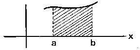
Figure: i051360a
The calculation of many quantities encountered in practice reduces to the problem of calculating the limit of integral sums; in other words, finding a definite integral; for example, areas of figures and surfaces, volumes of bodies, work done by force, the coordinates of the centre of gravity, the values of the moments of inertia of various bodies, etc.
The definite integral is linear: If two functions $ f _ {1} $ and $ f _ {2} $ are integrable on an interval $ [ a , b ] $, then for any real numbers $ \lambda _ {1} $ and $ \lambda _ {2} $ the function
$$ \lambda _ {1} f _ {1} + \lambda _ {2} f _ {2} $$
is also integrable on this interval and
$$ \int\limits _ { a } ^ { b } [ \lambda _ {1} f _ {1} ( x) + \lambda _ {2} f _ {2} ( x) ] d x = \ \lambda _ {1} \int\limits _ { a } ^ { b } f _ {1} ( x) d x + \lambda _ {2} \int\limits _ { a } ^ { b } f _ {2} ( x) d x . $$
Integration of a function over an interval has the property of monotonicity: If the function $ f $ is integrable on the interval $ [ a , b ] $ and if $ [ c , d ] \subset [ a , b ] $, then $ f $ is integrable on $ [ c , d ] $ as well. The integral is also additive with respect to the intervals over which the integration is carried out: If $ a < c < b $ and the function $ f $ is integrable on the intervals $ [ a , c ] $ and $ [ c , b ] $, then it is integrable on $ [ a , b ] $, and
$$ \int\limits _ { a } ^ { b } f ( x) d x = \ \int\limits _ { a } ^ { c } f ( x) d x + \int\limits _ { c } ^ { b } f ( x) d x . $$
If $ f $ and $ g $ are Riemann integrable, then their product is also Riemann integrable. If $ f \geq g $ on $ [ a , b ] $, then
$$ \int\limits _ { a } ^ { b } f ( x) d x \geq \ \int\limits _ { a } ^ { b } g ( x) d x . $$
If $ f $ is integrable on $ [ a , b ] $, then the absolute value $ | f | $ is also integrable on $ [ a , b ] $ if $ - \infty < a < b < \infty $, and
$$ \left | \int\limits _ { a } ^ { b } f ( x) d x \ \right | \leq \ \int\limits _ { a } ^ { b } | f ( x) | d x . $$
By definition one sets
$$ \int\limits _ { a } ^ { a } f ( x) d x = 0 \ \ \textrm{ and } \ \ \int\limits _ { b } ^ { a } f ( x) d x = - \int\limits _ { a } ^ { b } f ( x) d x ,\ \ a < b . $$
A mean-value theorem holds for integrals. For example, if $ f $ and $ g $ are Riemann integrable on an interval $ [ a , b ] $, if $ m \leq f ( x) \leq M $, $ x \in [ a , b ] $, and if $ g $ does not change sign on $ [ a , b ] $, that is, it is either non-negative or non-positive throughout this interval, then there exists a number $ m \leq \mu \leq M $ for which
$$ \int\limits _ { a } ^ { b } f ( x) g ( x) d x = \mu \int\limits _ { a } ^ { b } g ( x) d x . $$
Under the additional hypothesis that $ f $ is continuous on $ [ a , b ] $, there exists in $ ( a , b ) $ a point $ \xi $ for which
$$ \int\limits _ { a } ^ { b } f ( x) g ( x) d x = \ f ( \xi ) \int\limits _ { a } ^ { b } g ( x) d x . $$
In particular, if $ g ( x) \equiv 1 $, then
$$ \int\limits _ { a } ^ { b } f ( x) d x = f ( \xi ) ( b - a ) . $$
Integrals with a variable upper limit.
If a function $ f $ is Riemann integrable on an interval $ [ a , b ] $, then the function $ F $ defined by
$$ F ( x) = \int\limits _ { a } ^ { x } f ( t) d t ,\ \ a \leq x \leq b , $$
is continuous on this interval. If, in addition, $ f $ is continuous at a point $ x _ {0} $, then $ F $ is differentiable at this point and $ F ^ { \prime } ( x _ {0} ) = f( x _ {0} ) $. In other words, at the points of continuity of a function the following formula holds:
$$ \frac{d}{dx} \int\limits _ { a } ^ { x } f ( t) d t = \ f ( x) . $$
Consequently, this formula holds for every Riemann-integrable function on an interval $ [ a , b ] $, except perhaps at a set of points having Lebesgue measure zero, since if a function is Riemann integrable on some interval, then its set of points of discontinuity has measure zero. Thus, if the function $ f $ is continuous on $ [ a , b ] $, then the function $ F $ defined by
$$ F ( x) = \int\limits _ { a } ^ { x } f ( t) d t $$
is a primitive of $ f $ on this interval. This theorem shows that the operation of differentiation is inverse to that of taking the definite integral with a variable upper limit, and in this way a relationship is established between definite and indefinite integrals:
$$ \int\limits f ( x) d x = \ \int\limits _ { a } ^ { x } f ( t) d t + C . $$
The geometric meaning of this relationship is that the problem of finding the tangent to a curve and the calculation of the area of plane figures are inverse operations in the above sense.
The following Newton–Leibniz formula holds for any primitive $ F $ of an integrable function $ f $ on an interval $ [ a , b] $:
$$ \int\limits _ { a } ^ { b } f ( x) d x = F ( b) - F ( a) . $$
It shows that the definite integral of a continuous function over some interval is equal to the difference of the values at the end points of this interval of any primitive of it. This formula is sometimes taken as the definition of the definite integral. Then it is proved that the integral $ \int _ {a} ^ {b} f ( x) d x $ introduced in this way is equal to the limit of the corresponding integral sums.
For definite integrals, the formulas for change of variables and integration by parts hold. Suppose, for example, that the function $ f $ is continuous on the interval $ ( a , b ) $ and that $ \phi $ is continuous together with its derivative $ \phi ^ \prime $ on the interval $ ( \alpha , \beta ) $, where $ ( \alpha , \beta ) $ is mapped by $ \phi $ into $ ( a , b ) $: $ a < \phi ( t) < b $ for $ \alpha < t < \beta $, so that the composite $ f \circ \phi $ is meaningful in $ ( \alpha , \beta ) $. Then, for $ \alpha _ {0} , \beta _ {0} \in ( \alpha , \beta ) $, the following formulas for change of variables holds:
$$ \int\limits _ { \phi ( \alpha _ {0} ) } ^ { \phi ( \beta _ {0} ) } f ( x) d x = \ \int\limits _ {\alpha _ {0} } ^ { {\beta _ 0 } } f [ \phi ( t) ] \phi ^ \prime ( t) d t . $$
The formula for integration by parts is:
$$ \int\limits _ { a } ^ { b } u ( x) d v ( x) = \ \left . u ( x) v ( x) \right | _ {x=} a ^ {x=} b - \int\limits _ { a } ^ { b } v ( x) d u ( x) , $$
where the functions $ u $ and $ v $ have Riemann-integrable derivatives on $ [ a , b ] $.
The Newton–Leibniz formula reduces the calculation of an indefinite integral to finding the values of its primitive. Since the problem of finding a primitive is intrinsically a difficult one, other methods of finding definite integrals are of great importance, among which one should mention the method of residues (cf. Residue of an analytic function; Complex integration, method of) and the method of differentiation or integration with respect to the parameter of a parameter-dependent integral. Numerical methods for the approximate computation of integrals have also been developed.
Generalizing the notion of an integral to the case of unbounded functions and to the case of an unbounded interval leads to the notion of the improper integral, which is defined by yet one more limit transition.
The notions of the indefinite and the definite integral carry over to complex-valued functions. The representation of any holomorphic function of a complex variable in the form of a Cauchy integral over a contour played an important role in the development of the theory of analytic functions.
The generalization of the notion of the definite integral of a function of a single variable to the case of a function of several variables leads to the notion of a multiple integral.
For unbounded sets and unbounded functions of several variables, one is led to the notion of the improper integral, as in the one-dimensional case.
The extension of the practical applications of integral calculus necessitated the introduction of the notions of the curvilinear integral, i.e. the integral along a curve, the surface integral, i.e. the integral over a surface, and more generally, the integral over a manifold, which are reducible in some sense to a definite integral (the curvilinear integral reduces to an integral over an interval, the surface integral to an integral over a (plane) region, the integral over an $ n $- dimensional manifold to an integral over an $ n $- dimensional region). Integrals over manifolds, in particular curvilinear and surface integrals, play an important role in the integral calculus of functions of several variables; by this means a relationship is established between integration over a region and integration over its boundary or, in the general case, over a manifold and its boundary. This relationship is established by the Stokes formula (see also Ostrogradski formula; Green formulas), which is a generalization of the Newton–Leibniz formula to the multi-dimensional case.
Multiple, curvilinear and surface integrals find direct application in mathematical physics, particularly in field theory. Multiple integrals and concepts related to them are widely used in the solution of specific applied problems. The theory of cubature formulas (cf. Cubature formula) has been developed for the numerical calculation of multiple integrals.
The theory and methods of integral calculus of real- or complex-valued functions of a finite number of real or complex variables carry over to more general objects. For example, the theory of integration of functions whose values lie in a normed linear space, functions defined on topological groups, generalized functions, and functions of an infinite number of variables (integrals over trajectories). Finally, a new direction in integral calculus is related to the emergence and development of constructive mathematics.
Integral calculus is applied in many branches of mathematics (in the theory of differential and integral equations, in probability theory and mathematical statistics, in the theory of optimal processes, etc.), and in applications of it. For references see also [1]– to Differential calculus.
References
| [1] | I.L. Heiberg (ed.) , Archimedes: Opera Omnia , Wissenschaft. Buchgesellschaft , Darmstadt (1972) |
| [2] | W. von Dyk (ed.) M. Caspar (ed.) , J. Keppler: Gesammelte Werke , C.H. Beck (1937) |
| [3] | B. Cavalieri, "Geometria indivisibilibus (continuorum nova quadam ratione promota)" , Bologna (1635) |
| [4] | L. Euler, "Integralrechnung" , Berlin (1770) |
Comments
See also Infinitesimal calculus.
References
| [a1] | G. Valiron, "Théorie des fonctions" , Masson (1948) |
| [a2] | T.M. Apostol, "Calculus" , 1–2 , Blaisdell (1969) |
| [a3] | T.M. Apostol, "Mathematical analysis" , Addison-Wesley (1963) |
| [a4] | W. Rudin, "Real and complex analysis" , McGraw-Hill (1974) pp. 24 |
| [a5] | A.C. Zaanen, "Integration" , North-Holland (1967) |
| [a6] | W.M. Priestley, "Calculus: a historical approach" , Springer (1979) |
Integral calculus. Encyclopedia of Mathematics. URL: http://encyclopediaofmath.org/index.php?title=Integral_calculus&oldid=14758