Difference between revisions of "Dantzig-Wolfe decomposition"
(Importing text file) |
(latex details) |
||
| (3 intermediate revisions by 2 users not shown) | |||
| Line 1: | Line 1: | ||
| + | <!--This article has been texified automatically. Since there was no Nroff source code for this article, | ||
| + | the semi-automatic procedure described at https://encyclopediaofmath.org/wiki/User:Maximilian_Janisch/latexlist | ||
| + | was used. | ||
| + | If the TeX and formula formatting is correct and if all png images have been replaced by TeX code, please remove this message and the {{TEX|semi-auto}} category. | ||
| + | |||
| + | Out of 276 formulas, 255 were replaced by TEX code.--> | ||
| + | |||
| + | {{TEX|semi-auto}}{{TEX|part}} | ||
''Dantzig–Wolfe decomposition algorithm'' | ''Dantzig–Wolfe decomposition algorithm'' | ||
Consider the following [[Linear programming|linear programming]] problem (LP problem), with a row structure as indicated by the two sets of constraints. | Consider the following [[Linear programming|linear programming]] problem (LP problem), with a row structure as indicated by the two sets of constraints. | ||
| − | + | \begin{equation*} ( \text{P} ) v ^ { * } = \left\{ \begin{array} { c c } { \operatorname { min } } & { c ^ { T } x } \\ { \text { s.t. } } & { A _ { 1 } x \leq b _ { 1 }, } \\ { } & { A _ { 2 } x \leq b _ { 2 }, } \\ {} & { x \geq 0. } \end{array} \right. \end{equation*} | |
| − | The Dantzig–Wolfe approach is often used for the case when | + | The Dantzig–Wolfe approach is often used for the case when $( \text{P} )$ is a block-angular (linear) programming problem. Then the second constraint set $A _ { 2 } x \leq b _ { 2 }$ is separable into a number of parts, containing disjoint sets of variables. |
| − | The optimal solution is usually denoted by | + | The optimal solution is usually denoted by $x ^ { * }$. One denotes the LP-dual of $( \text{P} )$ by $( \operatorname{PD} )$ and the optimal dual solution by $( u _ { 1 } ^ { * } , u _ { 2 } ^ { * } )$. |
| − | The row structure can be utilized by applying Lagrangean duality to the first constraint set | + | The row structure can be utilized by applying Lagrangean duality to the first constraint set $A _ { 1 } x \leq b _ { 1 }$: |
| − | + | \begin{equation*} ( \operatorname{L} ) v ^ { * } = \left\{ \begin{array} { l l } { \operatorname { max } } & { g ( u _ { 1 } ) } \\ { s.t. } & { u _ { 1 } \in U _ { 1 }, } \end{array} \right. \end{equation*} | |
| − | where, for any fixed | + | where, for any fixed $\overline { u } _ { 1 } \in U _ { 1 }$, |
| − | + | \begin{equation*} ( \text{S} ) g ( \overline { u } _ { 1 } ) = \left\{ \begin{array} { c l } { \operatorname { min } } & { c ^ { T } x + \overline { u } _{1} ^ { T } ( A _ { 1 } x - b _ { 1 } ) } \\ { \text { s.t. } } & { A _ { 2 } x \leq b _ { 2 }, } \\ { } & { x \geq 0, } \end{array} \right. \end{equation*} | |
| − | and | + | and $U _ { 1 } = \{ u _ { 1 } \geq 0 : g ( u _ { 1 } ) > - \infty \}$. |
| − | + | $( \operatorname{S} )$ is called the subproblem and must be solved in order to evaluate the dual function $g ( u _ { 1 } )$ at a certain point, $\overline { u } _ { 1 } \in U _ { 1 }$. | |
| − | One can show that | + | One can show that $g ( u _ { 1 } ) \leq v ^ { * }$ for all $u _ { 1 } \geq 0$. The controllability of the subproblem is limited. Inserting $\overline { u } _ { 1 } = u _ { 1 } ^ { * }$ in $( \operatorname{S} )$ yields $u _ { 2 } = u _ { 2 } ^ { * }$, but possibly not $x = x ^ { * }$. |
| − | + | $U _ { 1 }$ is the region where $( \operatorname{S} )$ is bounded, i.e. where its dual is feasible, leading to <img align="absmiddle" border="0" src="https://www.encyclopediaofmath.org/legacyimages/d/d120/d120020/d12002024.png"/>. | |
| − | Now, let | + | Now, let $X = \{ x : A _ { 2 } x \leq b _ { 2 } , x \geq 0 \}$, which is the feasible set of $( \operatorname{S} )$. Since $X$ is a [[Polyhedron|polyhedron]], it has a finite number of extreme points, $x ^ { ( k ) }$, $k \in P$, and extreme rays, $\tilde{x} ^ { ( k ) }$, $k \in R$. Any point in $X$ can be described as |
| − | + | \begin{equation} \tag{a1} v ^ { * } = \sum _ { k \in P } \lambda _ { k } x ^ { ( k ) } + \sum _ { k \in R } \mu _ { k } \tilde{x} ^ { ( k ) }, \end{equation} | |
| − | where | + | where $\sum _ { k \in P } \lambda _ { k } = 1$, $\lambda _ { k } \geq 0$ for all $k \in P$ and $\mu _ { k } \geq 0$ for all $k \in R$. If $\overline { u } _ { 1 } \in U _ { 1 }$, then the optimal solution of $( \operatorname{S} )$ is bounded, and since $( \operatorname{S} )$ is a linear programming problem, the optimum is clearly attained in one of the extreme points $x ^ { ( k ) }$ of $X$. So, |
| − | + | \begin{equation*} g ( u _ { 1 } ) = \end{equation*} | |
| − | + | \begin{equation*} = \operatorname { min } _ { x \in X } c ^ { T } x + u _ { 1 } ^ { T } ( A _ { 1 } x - b _ { 1 } ) = \end{equation*} | |
| − | + | \begin{equation*} = \operatorname { min } _ { k \in P } c ^ { T } x ^ { ( k ) } + u _ { 1 } ^ { T } ( A _ { 1 } x ^ { ( k ) } - b _ { 1 } ). \end{equation*} | |
| − | Also, it is sufficient to include the extreme directions, yielding | + | Also, it is sufficient to include the extreme directions, yielding $U _ { 1 } = \{ u _ { 1 } \geq 0 : c ^ { T } \tilde { x } ^{ ( k ) } + u _ { 1 } A _ { 1 } \tilde{x} ^ { ( k ) } \geq 0 \text { for all } k \in R \}$. |
| − | These descriptions of | + | These descriptions of $g ( u _ { 1 } )$ and $U _ { 1 }$ can be used to form a problem that is (by construction) equivalent to $( \text{L} )$, in the sense that $q = v ^ { * }$ and $u _ { 1 } = u _ { 1 } ^ { * }$ is an optimal solution: |
| − | + | \begin{equation*} ( \text{LD} ) v ^ { * } = \left\{ \begin{array} { c l } { \operatorname { max } } & { q } \\ { s.t. } & { q \leq c ^ { T } x ^ { ( k ) } + u _ { 1 } ^ { T } ( A _ { 1 } x ^ { ( k ) } - b _ { 1 } ), } \\ { } & { \forall k \in P, } \\ { 0 \leq } & { c ^ { T } \tilde{x} ^ { ( k ) } + u _ { 1 } ^ { T } A _ { 1 } \tilde{x} ^ { ( k ) } , \forall k \in R, } \\ { u _ { 1 } \geq 0. } \end{array} \right. \end{equation*} | |
| − | The dual variables of the first and second constraints in | + | The dual variables of the first and second constraints in $( \text{P} )$ are actually the weights $\lambda _ { k }$ and $\mu _ { k }$ used above, so the LP-dual of $( \operatorname {LD} )$ is as given below: |
| − | <table class="eq" style="width:100%;"> <tr><td | + | <table class="eq" style="width:100%;"> <tr><td style="width:94%;text-align:center;" valign="top"><img align="absmiddle" border="0" src="https://www.encyclopediaofmath.org/legacyimages/d/d120/d120020/d12002058.png"/></td> </tr></table> |
| − | + | $( \operatorname{LP} )$ can be directly obtained from $( \text{P} )$ by doing the substitution (a1) above. | |
| − | If | + | If $( \overline { \lambda } , \overline { \mu } )$ is optimal in $( \operatorname{LP} )$, then $\overline{x} = \sum _ { k \in P } \overline { \lambda } _ { k } x ^ { ( k ) } + \sum _ { k \in R } \overline { \mu } _ { k } \tilde{x} ^ { ( k ) }$ is optimal in $( \text{P} )$. |
| − | The number of extreme points, | + | The number of extreme points, $| P |$, and the number of extreme directions, $| R |$, are generally very large, so in most cases $( \operatorname{LP} )$ is too large to be solved directly with a linear programming code. Therefore one solves $( \operatorname{LP} )$ with column generation. An approximation of $( \operatorname{LP} )$ is obtained by including only a subset of the variables. Let $P ^ { \prime } \subseteq P$ and $R ^ { \prime } \subseteq R$ be indices of extreme points and extreme directions that are included. |
| − | Replacing | + | Replacing $P$ by $P ^ { \prime }$ and $R$ by $R ^ { \prime }$ in $( \operatorname {LD} )$ yields the restricted master problem or the Dantzig–Wolfe master problem, $( \operatorname { M} )$, with objective function value <img align="absmiddle" border="0" src="https://www.encyclopediaofmath.org/legacyimages/d/d120/d120020/d12002078.png"/>. Doing the same in $( \operatorname{LP} )$ yields the problem $( \operatorname{MP} )$. The constraints of $( \operatorname { M} )$ are called dual value cuts and dual feasibility cuts. $( \operatorname { M} )$ can have the same optimal $u_1$-solution as $( \operatorname {LD} )$ (and thus as $( \operatorname{PD} )$) even if a large number of unnecessary dual cuts are missing. If the descriptions of $g ( u _ { 1 } )$ or $U _ { 1 }$ are insufficient at $u_{1}^{*}$, the solution obtained will violate at least one of the missing cuts. Since $( \operatorname { M} )$ is obtained from $( \operatorname {LD} )$ by simply dropping a number of constraints, it is easy to see that $v _ { \operatorname{M} } \geq v ^ { * }$ and that $v _ { \text{M} }$ will converge towards <img align="absmiddle" border="0" src="https://www.encyclopediaofmath.org/legacyimages/d/d120/d120020/d12002093.png"/> if the sets of cuts grow towards $P$ and $R$. |
| − | Since | + | Since $( \operatorname{LP} )$ is a linear programming problem, one can calculate the reduced cost for each variable, $\hat{c} ^ { 1_k } $, $k \in P$, and $\hat { c } ^ { 2 }_k$, $k \in R$, for a certain basic solution of $( \operatorname{LP} )$, i.e. for a certain dual solution, denoted by $\overline { u }_1$ and $\overline { q }$, as |
| − | + | \begin{equation*} \hat { c } _ { k } ^ { 1 } = c ^ { T } x ^ { ( k ) } + ( A _ { 1 } x ^ { ( k ) } - b _ { 1 } ) ^ { T } \overline { u } _ { 1 } - \overline { q }, \end{equation*} | |
| − | <table class="eq" style="width:100%;"> <tr><td | + | <table class="eq" style="width:100%;"> <tr><td style="width:94%;text-align:center;" valign="top"><img align="absmiddle" border="0" src="https://www.encyclopediaofmath.org/legacyimages/d/d120/d120020/d120020105.png"/></td> </tr></table> |
| − | + | $( \operatorname{LP} )$ is a minimization problem, so the optimum is reached if $\widehat { c } ^ { 1 } k \geq 0$ for all $k \in P$ and $\hat{c}_{k} ^ { 2 } \geq 0$ for all $k \in R$. A variable with a negative reduced cost can improve the solution, if it is entered into the basis. The variable with the most negative reduced cost can be found by | |
| − | <table class="eq" style="width:100%;"> <tr><td | + | <table class="eq" style="width:100%;"> <tr><td style="width:94%;text-align:center;" valign="top"><img align="absmiddle" border="0" src="https://www.encyclopediaofmath.org/legacyimages/d/d120/d120020/d120020111.png"/></td> </tr></table> |
| − | <table class="eq" style="width:100%;"> <tr><td | + | <table class="eq" style="width:100%;"> <tr><td style="width:94%;text-align:center;" valign="top"><img align="absmiddle" border="0" src="https://www.encyclopediaofmath.org/legacyimages/d/d120/d120020/d120020112.png"/></td> </tr></table> |
| − | Both of these, and the least of them, can be found by solving the dual subproblem | + | Both of these, and the least of them, can be found by solving the dual subproblem $( \operatorname{S} )$. |
| − | So, if | + | So, if $( \operatorname{S} )$ has a bounded solution, $x ^ { ( l ) }$, this yields a $\lambda_{l}$-variable that should enter the basis if <img align="absmiddle" border="0" src="https://www.encyclopediaofmath.org/legacyimages/d/d120/d120020/d120020117.png"/>. If $( \operatorname{S} )$ has an unbounded solution, $\tilde{x} ^ { ( l ) }$, this yields a $\mu_{l}$-variable, that should enter the basis if $\hat { c } _ { l } ^ { 2 } < 0$. |
| − | The | + | The $\lambda_{l}$-variable should enter the basis if $\hat { c } _ { l } ^ { 1 } = c ^ { T } x ^ { ( l ) } + ( A _ { 1 } x ^ { ( l ) } - b _ { 1 } ) ^ { T } \overline { u } _ { 1 } - \overline { q } < 0$. $\overline { q }$ is the objective function value of $( \operatorname{LP} )$ at the present basis, which might not be optimal, so $\overline { q } \geq v ^ { * }$. Secondly, $g ( \overline { u } _ { 1 } ) = c ^ { T } x ^ { ( l ) } + ( A _ { 1 } x ^ { ( l ) } - b _ { 1 } ) ^ { T } \overline { u _1}$, which is the optimal objective function value of $( \operatorname{S} )$, and $g ( u _ { 1 } ) \leq v ^ { * }$. Thus, |
| − | <table class="eq" style="width:100%;"> <tr><td | + | <table class="eq" style="width:100%;"> <tr><td style="width:94%;text-align:center;" valign="top"><img align="absmiddle" border="0" src="https://www.encyclopediaofmath.org/legacyimages/d/d120/d120020/d120020130.png"/></td> </tr></table> |
| − | + | \begin{equation*} = g ( \overline { u } _ { 1 } ) - \overline { q } = g ( \overline { u } _ { 1 } ) - v _ { \text{M} }, \end{equation*} | |
| − | and since | + | and since $g ( \overline { u } _ { 1 } ) \leq v ^ { * } \leq \overline { q }$, $\hat{c}_{k}^{1} \leq 0$. Equality is only possible if $g ( \overline { u } _ { 1 } ) = v ^ { * } = \overline { q } = v _ { \text{M} }$, i.e. if the present basis is optimal. In other words, the existence of a variable $\lambda_{l}$ with $\hat { c }_k^1< 0$ is equivalent to the lower bound obtained from the subproblem being strictly less than the upper bound obtained from the master problem. |
| − | Finding variables with negative reduced costs to introduce into the basis in | + | Finding variables with negative reduced costs to introduce into the basis in $( \operatorname{LP} )$ (i.e. to introduce in $( \operatorname{MP} )$) can thus be done by solving $( \operatorname{S} )$, since $( \operatorname{LP} )$ yields the column with the most negative reduced cost (or the most violated cut of $( \operatorname {LD} )$). This forms the basis of the Dantzig–Wolfe algorithm. |
| − | In the [[Simplex method|simplex method]], the entering variable does not need to be the one with the most negative reduced cost. Any negative reduced cost suffices. This means that instead of solving | + | In the [[Simplex method|simplex method]], the entering variable does not need to be the one with the most negative reduced cost. Any negative reduced cost suffices. This means that instead of solving $( \operatorname{S} )$ to optimality, it can be sufficient to either find a direction $\tilde{x}$ of $X$ such that <img align="absmiddle" border="0" src="https://www.encyclopediaofmath.org/legacyimages/d/d120/d120020/d120020145.png"/>, or a point $\bar{x}$ in $X$ such that $c ^ { T } \overline{x} + \overline { u } _1^ { T } ( A _ { 1 } \overline{x} - b _ { 1 } ) < \overline { q }$. |
| − | In the Dantzig–Wolfe decomposition algorithm, there might occur unbounded dual solutions to | + | In the Dantzig–Wolfe decomposition algorithm, there might occur unbounded dual solutions to $( \operatorname { M} )$. They can generate information about $g ( u _ { 1 } )$ and $U _ { 1 }$ (i.e. generate cuts for $( \operatorname { M} )$ or columns for $( \operatorname{MP} )$), or they can be optimal in $( \operatorname{PD} )$ (when $( \text{P} )$ is infeasible). The modified subproblem that accepts an unbounded solution as input (and yields a cut that eliminates it, unless it is optimal in $( \operatorname{PD} )$) is as follows. Let the unbounded solution be the non-negative (extreme) direction $\tilde{u}_1$, |
| − | <table class="eq" style="width:100%;"> <tr><td | + | <table class="eq" style="width:100%;"> <tr><td style="width:94%;text-align:center;" valign="top"><img align="absmiddle" border="0" src="https://www.encyclopediaofmath.org/legacyimages/d/d120/d120020/d120020158.png"/></td> </tr></table> |
| − | Assume that | + | Assume that $\tilde{u} _ { 1 } \geq 0$, $\tilde{u} _ { 1 } \neq 0$, $X \neq \emptyset$ and that $( \operatorname{PD} )$ is feasible. Then $\tilde{v} ( \tilde { u } _ { 1 } ) > 0$ if and only if $( \text{P} )$ is infeasible and $\tilde{u}_1$ is a part of an unbounded solution of $( \operatorname{PD} )$. The algorithm should then be terminated. |
| − | Assume that | + | Assume that $\tilde{u} _ { 1 } \geq 0$. If $\tilde{v} ( \tilde{u} _ { 1 } ) \leq 0$ then $( \text{US} )$ will yield a cut for $( \operatorname { M} )$ that ensures that $\tilde{u}_1$ is not an unbounded solution of $( \operatorname { M} )$. |
| − | In the Dantzig–Wolfe algorithm, [[#References|[a1]]], one iterates between the dual subproblem, | + | In the Dantzig–Wolfe algorithm, [[#References|[a1]]], one iterates between the dual subproblem, $( \operatorname{S} )$ or $( \text{US} )$, and the dual master problem, $( \operatorname { M} )$ (or $( \operatorname{MP} )$). The master problem indicates if there are necessary extreme points or directions missing, and the subproblem generates such points and directions, i.e. the cuts or columns that are needed. Since there is only a finite number of possible cuts, this algorithm will converge to the exact optimum in a finite number of steps. |
| − | ==Algorithmic description of the Dantzig–Wolfe decomposition method for solving | + | ==Algorithmic description of the Dantzig–Wolfe decomposition method for solving $( \text{P} )$.== |
| − | 1) Generate a dual starting solution, | + | 1) Generate a dual starting solution, $\overline { u }_1$, and, optionally, a starting set of primal extreme solutions, $x ^ { ( k ) }$ and $\tilde{x} ^ { ( k ) }$. Initialize $P ^ { \prime }$, $R ^ { \prime }$, $\underline { v } = - \infty$ and $\overline { v } = \infty$. Set $k = 1$. |
| − | 2) Solve the dual subproblem | + | 2) Solve the dual subproblem $( \operatorname{S} )$ with $\overline { u }_1$. |
| − | If | + | If $( \operatorname{S} )$ is infeasible: Stop. $( \text{P} )$ is infeasible. |
| − | Else, a primal extreme solution is obtained: either a point | + | Else, a primal extreme solution is obtained: either a point $x ^ { ( k ) }$ and the value $g(\overline{u}_1)$ or a direction $\tilde{x} ^ { ( k ) }$. If $g ( \overline { u } _ { 1 } ) > \underline { v }$, set $\underline { v } = g ( \overline { u } _ { 1 } )$. Go to 4). |
| − | 3) Solve the dual subproblem | + | 3) Solve the dual subproblem $( \text{US} )$ with $\tilde{u}_1$. A primal extreme solution is obtained: either a point $x ^ { ( k ) }$ and the value $\tilde{v} ( \tilde { u } _ { 1 } )$ or a direction $\tilde{x} ^ { ( k ) }$. |
| − | If | + | If $\tilde{v} ( \tilde { u } _ { 1 } ) > 0$: Stop. $( \text{P} )$ is infeasible. Else, go to 5). |
| − | 4) Optimality test: If <img align="absmiddle" border="0" src="https://www.encyclopediaofmath.org/legacyimages/d/d120/d120020/d120020202.png" />, then go to 7). | + | 4) Optimality test: If <img align="absmiddle" border="0" src="https://www.encyclopediaofmath.org/legacyimages/d/d120/d120020/d120020202.png"/>, then go to 7). |
| − | 5) Solve the dual master problem | + | 5) Solve the dual master problem $( \operatorname { M} )$ (and $( \operatorname{MP} )$) with all the known primal solutions $x ^ { ( k ) }$, $k \in P ^ { \prime }$ and $\tilde{x} ^ { ( k ) }$, $k \in R ^ { \prime }$. |
| − | If | + | If $( \operatorname { M} )$ is infeasible: Stop. $( \text{P} )$ is unbounded. |
| − | Else, this yields | + | Else, this yields $( \overline { \lambda } , \overline { \mu } )$ and a new dual solution: either a point $\overline { u }_1$ and an upper bound <img align="absmiddle" border="0" src="https://www.encyclopediaofmath.org/legacyimages/d/d120/d120020/d120020213.png"/> or a direction $\tilde{u}_1$. |
| − | 6) Optimality test: If <img align="absmiddle" border="0" src="https://www.encyclopediaofmath.org/legacyimages/d/d120/d120020/d120020215.png" /> then go to 7). Else, set | + | 6) Optimality test: If <img align="absmiddle" border="0" src="https://www.encyclopediaofmath.org/legacyimages/d/d120/d120020/d120020215.png"/> then go to 7). Else, set $ k = k + 1$. |
| − | If the dual solution is a point, | + | If the dual solution is a point, $\overline { u }_1$, go to 2), and if it is a direction, $\tilde{u}_1$, go to 3). |
| − | 7) Stop. The optimal solution of | + | 7) Stop. The optimal solution of $( \text{P} )$ is $\overline{x} = \sum _ { k \in P ^ { \prime } } \overline { \lambda } _ { k } x ^ { ( k ) } + \sum _ { k \in R ^ { \prime } } \overline { \mu } _ { k } \tilde{x} ^ { ( k ) }$. |
===Comments.=== | ===Comments.=== | ||
| − | In step 5) one always sets <img align="absmiddle" border="0" src="https://www.encyclopediaofmath.org/legacyimages/d/d120/d120020/d120020221.png" /> because the objective function value of M) is decreasing (since in each iteration a constraint is added), but in step 2) one only sets | + | In step 5) one always sets <img align="absmiddle" border="0" src="https://www.encyclopediaofmath.org/legacyimages/d/d120/d120020/d120020221.png"/> because the objective function value of M) is decreasing (since in each iteration a constraint is added), but in step 2) one only sets $\underline { v } = g ( \overline { u } _ { 1 } )$ if this yields an increase in $\underline{v}$, since the increase in $g(\overline{u}_1)$ is probably not monotone. If $( \operatorname { M} )$ is infeasible, the direction of the unbounded solution of $( \text{P} )$ can be obtained from the unbounded solution of $( \operatorname{MP} )$ $\tilde{\pi}$ as $\tilde { x } = \sum _ { k \in R ^ { \prime } } \overline { \mu } _ { k }\, \tilde { x } ^ { ( k ) }$. |
===Convergence.=== | ===Convergence.=== | ||
The algorithm has finite convergence, as described below. | The algorithm has finite convergence, as described below. | ||
| − | Assume that | + | Assume that $( \text{P} )$ is feasible and that $\overline { u }_1$ is a solution of $( \operatorname { M} )$. Then $g ( \overline { u } _ { 1 } ) = v _ { M }$ if and only if $v _ { M } = v ^ { * }$ and $\overline { u }_1$ is a part of the optimal solution of $( \operatorname{PD} )$. If this is true and $( \overline { \lambda } , \overline { \mu } )$ is the solution of $( \operatorname{MP} )$, then $\overline{x} = \sum _ { k \in P ^ { \prime } } \overline { \lambda } _ { k } x ^ { ( k ) } + \sum _ { k \in R ^ { \prime } } \overline { \mu } _ { k } \tilde{x} ^ { ( k ) }$ is an optimal solution of $( \text{P} )$. |
| − | Assume that | + | Assume that $\overline { u } _ { 1 } \geq 0$. If $g ( \overline { u } _ { 1 } ) < v _ { M } = \overline { q }$, then $( \operatorname{S} )$ will yield a cut that ensures that ($\overline { u }_{ 1 } , \overline { q }$) is not a solution of $( \operatorname { M} )$. |
| − | It is important to know that | + | It is important to know that $( \operatorname{S} )$ and $( \text{US} )$ do not yield any solutions more than once (unless they are optimal). This depends on the inputs to $( \operatorname{S} )$ and $( \text{US} )$, $\overline { u }_1$ and $\tilde{u}_1$, which are obtained from the dual master problem, $( \operatorname { M} )$. |
| − | Assume that | + | Assume that $\overline { u } _ { 1 } \geq 0$ is a solution of $( \operatorname { M} )$. If $v _ { M } > v ^ { * }$, then solving $( \operatorname{S} )$ at $\overline { u }_1$ will yield a so far unknown cut that ensures that $( \operatorname { M} )$ will not have the same solution in the next iteration, i.e. $( \operatorname { M} )$ will yield either a different $u_1$-solution or the same, $\overline { u }_1$, with a lower value of $\overline { q }$ ($= v _ { M }$). |
| − | Assume that | + | Assume that $\tilde{u} _ { 1 } \geq 0$ is an unbounded solution of $( \operatorname { M} )$. Then solving $( \text{US} )$ at $\tilde{u}_1$ will yield a so far unknown cut that ensures that $( \operatorname { M} )$ will not have the same solution in the next iteration, or will prove that $( \text{P} )$ is infeasible. |
| − | All this shows that the Dantzig–Wolfe decomposition algorithm for solving | + | All this shows that the Dantzig–Wolfe decomposition algorithm for solving $( \text{P} )$ will terminate with the correct solution within a finite number of iterations. |
====References==== | ====References==== | ||
| − | <table>< | + | <table> |
| + | <tr><td valign="top">[a1]</td> <td valign="top"> G.B. Dantzig, P. Wolfe, "Decomposition principle for linear programs." ''Oper. Res.'' , '''8''' (1960) pp. 101–111</td></tr> | ||
| + | </table> | ||
Latest revision as of 16:39, 2 February 2024
Dantzig–Wolfe decomposition algorithm
Consider the following linear programming problem (LP problem), with a row structure as indicated by the two sets of constraints.
\begin{equation*} ( \text{P} ) v ^ { * } = \left\{ \begin{array} { c c } { \operatorname { min } } & { c ^ { T } x } \\ { \text { s.t. } } & { A _ { 1 } x \leq b _ { 1 }, } \\ { } & { A _ { 2 } x \leq b _ { 2 }, } \\ {} & { x \geq 0. } \end{array} \right. \end{equation*}
The Dantzig–Wolfe approach is often used for the case when $( \text{P} )$ is a block-angular (linear) programming problem. Then the second constraint set $A _ { 2 } x \leq b _ { 2 }$ is separable into a number of parts, containing disjoint sets of variables.
The optimal solution is usually denoted by $x ^ { * }$. One denotes the LP-dual of $( \text{P} )$ by $( \operatorname{PD} )$ and the optimal dual solution by $( u _ { 1 } ^ { * } , u _ { 2 } ^ { * } )$.
The row structure can be utilized by applying Lagrangean duality to the first constraint set $A _ { 1 } x \leq b _ { 1 }$:
\begin{equation*} ( \operatorname{L} ) v ^ { * } = \left\{ \begin{array} { l l } { \operatorname { max } } & { g ( u _ { 1 } ) } \\ { s.t. } & { u _ { 1 } \in U _ { 1 }, } \end{array} \right. \end{equation*}
where, for any fixed $\overline { u } _ { 1 } \in U _ { 1 }$,
\begin{equation*} ( \text{S} ) g ( \overline { u } _ { 1 } ) = \left\{ \begin{array} { c l } { \operatorname { min } } & { c ^ { T } x + \overline { u } _{1} ^ { T } ( A _ { 1 } x - b _ { 1 } ) } \\ { \text { s.t. } } & { A _ { 2 } x \leq b _ { 2 }, } \\ { } & { x \geq 0, } \end{array} \right. \end{equation*}
and $U _ { 1 } = \{ u _ { 1 } \geq 0 : g ( u _ { 1 } ) > - \infty \}$.
$( \operatorname{S} )$ is called the subproblem and must be solved in order to evaluate the dual function $g ( u _ { 1 } )$ at a certain point, $\overline { u } _ { 1 } \in U _ { 1 }$.
One can show that $g ( u _ { 1 } ) \leq v ^ { * }$ for all $u _ { 1 } \geq 0$. The controllability of the subproblem is limited. Inserting $\overline { u } _ { 1 } = u _ { 1 } ^ { * }$ in $( \operatorname{S} )$ yields $u _ { 2 } = u _ { 2 } ^ { * }$, but possibly not $x = x ^ { * }$.
$U _ { 1 }$ is the region where $( \operatorname{S} )$ is bounded, i.e. where its dual is feasible, leading to  .
.
Now, let $X = \{ x : A _ { 2 } x \leq b _ { 2 } , x \geq 0 \}$, which is the feasible set of $( \operatorname{S} )$. Since $X$ is a polyhedron, it has a finite number of extreme points, $x ^ { ( k ) }$, $k \in P$, and extreme rays, $\tilde{x} ^ { ( k ) }$, $k \in R$. Any point in $X$ can be described as
\begin{equation} \tag{a1} v ^ { * } = \sum _ { k \in P } \lambda _ { k } x ^ { ( k ) } + \sum _ { k \in R } \mu _ { k } \tilde{x} ^ { ( k ) }, \end{equation}
where $\sum _ { k \in P } \lambda _ { k } = 1$, $\lambda _ { k } \geq 0$ for all $k \in P$ and $\mu _ { k } \geq 0$ for all $k \in R$. If $\overline { u } _ { 1 } \in U _ { 1 }$, then the optimal solution of $( \operatorname{S} )$ is bounded, and since $( \operatorname{S} )$ is a linear programming problem, the optimum is clearly attained in one of the extreme points $x ^ { ( k ) }$ of $X$. So,
\begin{equation*} g ( u _ { 1 } ) = \end{equation*}
\begin{equation*} = \operatorname { min } _ { x \in X } c ^ { T } x + u _ { 1 } ^ { T } ( A _ { 1 } x - b _ { 1 } ) = \end{equation*}
\begin{equation*} = \operatorname { min } _ { k \in P } c ^ { T } x ^ { ( k ) } + u _ { 1 } ^ { T } ( A _ { 1 } x ^ { ( k ) } - b _ { 1 } ). \end{equation*}
Also, it is sufficient to include the extreme directions, yielding $U _ { 1 } = \{ u _ { 1 } \geq 0 : c ^ { T } \tilde { x } ^{ ( k ) } + u _ { 1 } A _ { 1 } \tilde{x} ^ { ( k ) } \geq 0 \text { for all } k \in R \}$.
These descriptions of $g ( u _ { 1 } )$ and $U _ { 1 }$ can be used to form a problem that is (by construction) equivalent to $( \text{L} )$, in the sense that $q = v ^ { * }$ and $u _ { 1 } = u _ { 1 } ^ { * }$ is an optimal solution:
\begin{equation*} ( \text{LD} ) v ^ { * } = \left\{ \begin{array} { c l } { \operatorname { max } } & { q } \\ { s.t. } & { q \leq c ^ { T } x ^ { ( k ) } + u _ { 1 } ^ { T } ( A _ { 1 } x ^ { ( k ) } - b _ { 1 } ), } \\ { } & { \forall k \in P, } \\ { 0 \leq } & { c ^ { T } \tilde{x} ^ { ( k ) } + u _ { 1 } ^ { T } A _ { 1 } \tilde{x} ^ { ( k ) } , \forall k \in R, } \\ { u _ { 1 } \geq 0. } \end{array} \right. \end{equation*}
The dual variables of the first and second constraints in $( \text{P} )$ are actually the weights $\lambda _ { k }$ and $\mu _ { k }$ used above, so the LP-dual of $( \operatorname {LD} )$ is as given below:
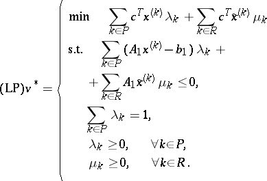 |
$( \operatorname{LP} )$ can be directly obtained from $( \text{P} )$ by doing the substitution (a1) above.
If $( \overline { \lambda } , \overline { \mu } )$ is optimal in $( \operatorname{LP} )$, then $\overline{x} = \sum _ { k \in P } \overline { \lambda } _ { k } x ^ { ( k ) } + \sum _ { k \in R } \overline { \mu } _ { k } \tilde{x} ^ { ( k ) }$ is optimal in $( \text{P} )$.
The number of extreme points, $| P |$, and the number of extreme directions, $| R |$, are generally very large, so in most cases $( \operatorname{LP} )$ is too large to be solved directly with a linear programming code. Therefore one solves $( \operatorname{LP} )$ with column generation. An approximation of $( \operatorname{LP} )$ is obtained by including only a subset of the variables. Let $P ^ { \prime } \subseteq P$ and $R ^ { \prime } \subseteq R$ be indices of extreme points and extreme directions that are included.
Replacing $P$ by $P ^ { \prime }$ and $R$ by $R ^ { \prime }$ in $( \operatorname {LD} )$ yields the restricted master problem or the Dantzig–Wolfe master problem, $( \operatorname { M} )$, with objective function value  . Doing the same in $( \operatorname{LP} )$ yields the problem $( \operatorname{MP} )$. The constraints of $( \operatorname { M} )$ are called dual value cuts and dual feasibility cuts. $( \operatorname { M} )$ can have the same optimal $u_1$-solution as $( \operatorname {LD} )$ (and thus as $( \operatorname{PD} )$) even if a large number of unnecessary dual cuts are missing. If the descriptions of $g ( u _ { 1 } )$ or $U _ { 1 }$ are insufficient at $u_{1}^{*}$, the solution obtained will violate at least one of the missing cuts. Since $( \operatorname { M} )$ is obtained from $( \operatorname {LD} )$ by simply dropping a number of constraints, it is easy to see that $v _ { \operatorname{M} } \geq v ^ { * }$ and that $v _ { \text{M} }$ will converge towards
  if the sets of cuts grow towards $P$ and $R$.
Since $( \operatorname{LP} )$ is a linear programming problem, one can calculate the reduced cost for each variable, $\hat{c} ^ { 1_k } $, $k \in P$, and $\hat { c } ^ { 2 }_k$, $k \in R$, for a certain basic solution of $( \operatorname{LP} )$, i.e. for a certain dual solution, denoted by $\overline { u }_1$ and $\overline { q }$, as
\begin{equation*} \hat { c } _ { k } ^ { 1 } = c ^ { T } x ^ { ( k ) } + ( A _ { 1 } x ^ { ( k ) } - b _ { 1 } ) ^ { T } \overline { u } _ { 1 } - \overline { q }, \end{equation*}
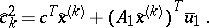 |
$( \operatorname{LP} )$ is a minimization problem, so the optimum is reached if $\widehat { c } ^ { 1 } k \geq 0$ for all $k \in P$ and $\hat{c}_{k} ^ { 2 } \geq 0$ for all $k \in R$. A variable with a negative reduced cost can improve the solution, if it is entered into the basis. The variable with the most negative reduced cost can be found by
 |
 |
Both of these, and the least of them, can be found by solving the dual subproblem $( \operatorname{S} )$.
So, if $( \operatorname{S} )$ has a bounded solution, $x ^ { ( l ) }$, this yields a $\lambda_{l}$-variable that should enter the basis if  . If $( \operatorname{S} )$ has an unbounded solution, $\tilde{x} ^ { ( l ) }$, this yields a $\mu_{l}$-variable, that should enter the basis if $\hat { c } _ { l } ^ { 2 } < 0$.
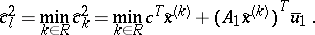
The $\lambda_{l}$-variable should enter the basis if $\hat { c } _ { l } ^ { 1 } = c ^ { T } x ^ { ( l ) } + ( A _ { 1 } x ^ { ( l ) } - b _ { 1 } ) ^ { T } \overline { u } _ { 1 } - \overline { q } < 0$. $\overline { q }$ is the objective function value of $( \operatorname{LP} )$ at the present basis, which might not be optimal, so $\overline { q } \geq v ^ { * }$. Secondly, $g ( \overline { u } _ { 1 } ) = c ^ { T } x ^ { ( l ) } + ( A _ { 1 } x ^ { ( l ) } - b _ { 1 } ) ^ { T } \overline { u _1}$, which is the optimal objective function value of $( \operatorname{S} )$, and $g ( u _ { 1 } ) \leq v ^ { * }$. Thus,
 |
\begin{equation*} = g ( \overline { u } _ { 1 } ) - \overline { q } = g ( \overline { u } _ { 1 } ) - v _ { \text{M} }, \end{equation*}
and since $g ( \overline { u } _ { 1 } ) \leq v ^ { * } \leq \overline { q }$, $\hat{c}_{k}^{1} \leq 0$. Equality is only possible if $g ( \overline { u } _ { 1 } ) = v ^ { * } = \overline { q } = v _ { \text{M} }$, i.e. if the present basis is optimal. In other words, the existence of a variable $\lambda_{l}$ with $\hat { c }_k^1< 0$ is equivalent to the lower bound obtained from the subproblem being strictly less than the upper bound obtained from the master problem.
Finding variables with negative reduced costs to introduce into the basis in $( \operatorname{LP} )$ (i.e. to introduce in $( \operatorname{MP} )$) can thus be done by solving $( \operatorname{S} )$, since $( \operatorname{LP} )$ yields the column with the most negative reduced cost (or the most violated cut of $( \operatorname {LD} )$). This forms the basis of the Dantzig–Wolfe algorithm.
In the simplex method, the entering variable does not need to be the one with the most negative reduced cost. Any negative reduced cost suffices. This means that instead of solving $( \operatorname{S} )$ to optimality, it can be sufficient to either find a direction $\tilde{x}$ of $X$ such that 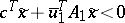 , or a point $\bar{x}$ in $X$ such that $c ^ { T } \overline{x} + \overline { u } _1^ { T } ( A _ { 1 } \overline{x} - b _ { 1 } ) < \overline { q }$.
In the Dantzig–Wolfe decomposition algorithm, there might occur unbounded dual solutions to $( \operatorname { M} )$. They can generate information about $g ( u _ { 1 } )$ and $U _ { 1 }$ (i.e. generate cuts for $( \operatorname { M} )$ or columns for $( \operatorname{MP} )$), or they can be optimal in $( \operatorname{PD} )$ (when $( \text{P} )$ is infeasible). The modified subproblem that accepts an unbounded solution as input (and yields a cut that eliminates it, unless it is optimal in $( \operatorname{PD} )$) is as follows. Let the unbounded solution be the non-negative (extreme) direction $\tilde{u}_1$,
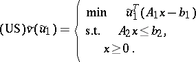 |
Assume that $\tilde{u} _ { 1 } \geq 0$, $\tilde{u} _ { 1 } \neq 0$, $X \neq \emptyset$ and that $( \operatorname{PD} )$ is feasible. Then $\tilde{v} ( \tilde { u } _ { 1 } ) > 0$ if and only if $( \text{P} )$ is infeasible and $\tilde{u}_1$ is a part of an unbounded solution of $( \operatorname{PD} )$. The algorithm should then be terminated.
Assume that $\tilde{u} _ { 1 } \geq 0$. If $\tilde{v} ( \tilde{u} _ { 1 } ) \leq 0$ then $( \text{US} )$ will yield a cut for $( \operatorname { M} )$ that ensures that $\tilde{u}_1$ is not an unbounded solution of $( \operatorname { M} )$.
In the Dantzig–Wolfe algorithm, [a1], one iterates between the dual subproblem, $( \operatorname{S} )$ or $( \text{US} )$, and the dual master problem, $( \operatorname { M} )$ (or $( \operatorname{MP} )$). The master problem indicates if there are necessary extreme points or directions missing, and the subproblem generates such points and directions, i.e. the cuts or columns that are needed. Since there is only a finite number of possible cuts, this algorithm will converge to the exact optimum in a finite number of steps.
Algorithmic description of the Dantzig–Wolfe decomposition method for solving $( \text{P} )$.
1) Generate a dual starting solution, $\overline { u }_1$, and, optionally, a starting set of primal extreme solutions, $x ^ { ( k ) }$ and $\tilde{x} ^ { ( k ) }$. Initialize $P ^ { \prime }$, $R ^ { \prime }$, $\underline { v } = - \infty$ and $\overline { v } = \infty$. Set $k = 1$.
2) Solve the dual subproblem $( \operatorname{S} )$ with $\overline { u }_1$.
If $( \operatorname{S} )$ is infeasible: Stop. $( \text{P} )$ is infeasible.
Else, a primal extreme solution is obtained: either a point $x ^ { ( k ) }$ and the value $g(\overline{u}_1)$ or a direction $\tilde{x} ^ { ( k ) }$. If $g ( \overline { u } _ { 1 } ) > \underline { v }$, set $\underline { v } = g ( \overline { u } _ { 1 } )$. Go to 4).
3) Solve the dual subproblem $( \text{US} )$ with $\tilde{u}_1$. A primal extreme solution is obtained: either a point $x ^ { ( k ) }$ and the value $\tilde{v} ( \tilde { u } _ { 1 } )$ or a direction $\tilde{x} ^ { ( k ) }$.
If $\tilde{v} ( \tilde { u } _ { 1 } ) > 0$: Stop. $( \text{P} )$ is infeasible. Else, go to 5).
4) Optimality test: If  , then go to 7).
5) Solve the dual master problem $( \operatorname { M} )$ (and $( \operatorname{MP} )$) with all the known primal solutions $x ^ { ( k ) }$, $k \in P ^ { \prime }$ and $\tilde{x} ^ { ( k ) }$, $k \in R ^ { \prime }$.
If $( \operatorname { M} )$ is infeasible: Stop. $( \text{P} )$ is unbounded.
Else, this yields $( \overline { \lambda } , \overline { \mu } )$ and a new dual solution: either a point $\overline { u }_1$ and an upper bound  or a direction $\tilde{u}_1$.
6) Optimality test: If  then go to 7). Else, set $ k = k + 1$.
If the dual solution is a point, $\overline { u }_1$, go to 2), and if it is a direction, $\tilde{u}_1$, go to 3).
7) Stop. The optimal solution of $( \text{P} )$ is $\overline{x} = \sum _ { k \in P ^ { \prime } } \overline { \lambda } _ { k } x ^ { ( k ) } + \sum _ { k \in R ^ { \prime } } \overline { \mu } _ { k } \tilde{x} ^ { ( k ) }$.
Comments.
In step 5) one always sets  because the objective function value of M) is decreasing (since in each iteration a constraint is added), but in step 2) one only sets $\underline { v } = g ( \overline { u } _ { 1 } )$ if this yields an increase in $\underline{v}$, since the increase in $g(\overline{u}_1)$ is probably not monotone. If $( \operatorname { M} )$ is infeasible, the direction of the unbounded solution of $( \text{P} )$ can be obtained from the unbounded solution of $( \operatorname{MP} )$ $\tilde{\pi}$ as $\tilde { x } = \sum _ { k \in R ^ { \prime } } \overline { \mu } _ { k }\, \tilde { x } ^ { ( k ) }$.
Convergence.
The algorithm has finite convergence, as described below.
Assume that $( \text{P} )$ is feasible and that $\overline { u }_1$ is a solution of $( \operatorname { M} )$. Then $g ( \overline { u } _ { 1 } ) = v _ { M }$ if and only if $v _ { M } = v ^ { * }$ and $\overline { u }_1$ is a part of the optimal solution of $( \operatorname{PD} )$. If this is true and $( \overline { \lambda } , \overline { \mu } )$ is the solution of $( \operatorname{MP} )$, then $\overline{x} = \sum _ { k \in P ^ { \prime } } \overline { \lambda } _ { k } x ^ { ( k ) } + \sum _ { k \in R ^ { \prime } } \overline { \mu } _ { k } \tilde{x} ^ { ( k ) }$ is an optimal solution of $( \text{P} )$.
Assume that $\overline { u } _ { 1 } \geq 0$. If $g ( \overline { u } _ { 1 } ) < v _ { M } = \overline { q }$, then $( \operatorname{S} )$ will yield a cut that ensures that ($\overline { u }_{ 1 } , \overline { q }$) is not a solution of $( \operatorname { M} )$.
It is important to know that $( \operatorname{S} )$ and $( \text{US} )$ do not yield any solutions more than once (unless they are optimal). This depends on the inputs to $( \operatorname{S} )$ and $( \text{US} )$, $\overline { u }_1$ and $\tilde{u}_1$, which are obtained from the dual master problem, $( \operatorname { M} )$.
Assume that $\overline { u } _ { 1 } \geq 0$ is a solution of $( \operatorname { M} )$. If $v _ { M } > v ^ { * }$, then solving $( \operatorname{S} )$ at $\overline { u }_1$ will yield a so far unknown cut that ensures that $( \operatorname { M} )$ will not have the same solution in the next iteration, i.e. $( \operatorname { M} )$ will yield either a different $u_1$-solution or the same, $\overline { u }_1$, with a lower value of $\overline { q }$ ($= v _ { M }$).
Assume that $\tilde{u} _ { 1 } \geq 0$ is an unbounded solution of $( \operatorname { M} )$. Then solving $( \text{US} )$ at $\tilde{u}_1$ will yield a so far unknown cut that ensures that $( \operatorname { M} )$ will not have the same solution in the next iteration, or will prove that $( \text{P} )$ is infeasible.
All this shows that the Dantzig–Wolfe decomposition algorithm for solving $( \text{P} )$ will terminate with the correct solution within a finite number of iterations.
References
| [a1] | G.B. Dantzig, P. Wolfe, "Decomposition principle for linear programs." Oper. Res. , 8 (1960) pp. 101–111 |
Dantzig-Wolfe decomposition. Encyclopedia of Mathematics. URL: http://encyclopediaofmath.org/index.php?title=Dantzig-Wolfe_decomposition&oldid=14930