Difference between revisions of "Bernoulli experiment"
(Importing text file) |
m (Automatically changed introduction) |
||
| (One intermediate revision by the same user not shown) | |||
| Line 1: | Line 1: | ||
| − | + | <!--This article has been texified automatically. Since there was no Nroff source code for this article, | |
| + | the semi-automatic procedure described at https://encyclopediaofmath.org/wiki/User:Maximilian_Janisch/latexlist | ||
| + | was used. | ||
| + | If the TeX and formula formatting is correct and if all png images have been replaced by TeX code, please remove this message and the {{TEX|semi-auto}} category. | ||
| − | + | Out of 169 formulas, 162 were replaced by TEX code.--> | |
| − | + | {{TEX|semi-auto}}{{TEX|part}} | |
| + | ''of size $n$'' | ||
| − | + | The special case of a statistical experiment $( \Omega , \mathcal{A} , \mathcal{P} )$ (cf. also [[Probability space|Probability space]]; [[Statistical experiments, method of|Statistical experiments, method of]]) consisting of a set $\mathcal{P}$ of probability measures $\mathsf{P}$ on a $\sigma$-algebra $\mathcal{A}$ of subsets of a set $\Omega$, where $\Omega = \{ 0,1 \} ^ { n }$ ($n \in \mathbf N$, $\mathbf{N}$ the set of natural numbers), $\mathcal{A}$ is the $\sigma$-algebra of all subsets of $\{ 0,1 \} ^ { n }$ and $\mathcal{P} = \{ \mathsf{P} _ { p } : p \in [ 0,1 ] \}$. Here, the [[Probability measure|probability measure]] $\mathsf{P} _ { p }$ describes the probability | |
| − | + | \begin{equation*} p^{\sum _ { j = 1 } ^ { n } x _ { j }} (1-p)^{ n - \sum _ { j = 1 } ^ { n } x _ { j }} \end{equation*} | |
| + | |||
| + | for a given probability $p \in [ 0,1 ]$ of success that $( x _ { 1 } , \dots , x _ { n } ) \in \{ 0,1 \} ^ { n }$ will be observed. Clearly, decision-theoretical procedures associated with Bernoulli experiments are based on the sum $\sum _ { j = 1 } ^ { n } x _ { j }$ of observations $( x _ { 1 } , \dots , x _ { n } ) \in \{ 0,1 \} ^ { n }$ because of the corresponding sufficient and complete data reduction (cf. [[#References|[a2]]] and [[#References|[a3]]]). Therefore, uniformly most powerful, as well as uniformly most powerful unbiased, level tests for one-sided and two-sided hypotheses about the probability $p$ of success are based on $\sum _ { j = 1 } ^ { n } x _ { j }$ (cf. [[#References|[a2]]]; see also [[Statistical hypotheses, verification of|Statistical hypotheses, verification of]]). Moreover, based on the quadratic loss function, the sample mean | ||
| + | |||
| + | \begin{equation*} \overline{x} = \frac { 1 } { n } \sum _ { j = 1 } ^ { n } x_{j} \end{equation*} | ||
is admissible on account of the [[Rao–Cramér inequality|Rao–Cramér inequality]] (cf. [[#References|[a3]]]) and the estimator (cf. also [[Statistical estimator|Statistical estimator]]) | is admissible on account of the [[Rao–Cramér inequality|Rao–Cramér inequality]] (cf. [[#References|[a3]]]) and the estimator (cf. also [[Statistical estimator|Statistical estimator]]) | ||
| − | + | \begin{equation*} \frac { 1 } { 1 + \sqrt { n } } \left( \bar{x} \sqrt { n } + \frac { 1 } { 2 } \right) \end{equation*} | |
| − | is minimax by means of equalizer decision rules (cf. [[#References|[a2]]]). Furthermore, the Lehmann–Scheffé theorem implies that | + | is minimax by means of equalizer decision rules (cf. [[#References|[a2]]]). Furthermore, the Lehmann–Scheffé theorem implies that $\bar{x}$ is a uniform minimum-variance unbiased estimator (an UMVU estimator; cf. also [[Unbiased estimator|Unbiased estimator]]) for the probability $p$ of success (cf. [[#References|[a2]]] and [[#References|[a3]]]). |
| − | All UMVU estimators, as well as all unbiased estimators of zero, might be characterized in connection with Bernoulli experiments by introducing the following notion for general statistical experiments | + | All UMVU estimators, as well as all unbiased estimators of zero, might be characterized in connection with Bernoulli experiments by introducing the following notion for general statistical experiments $( \Omega , \mathcal{A} , \mathcal{P} )$: A $d ^ { * } \in \cap_{ \mathsf{P} \in \mathcal{P}} L _ { 2 } ( \Omega , \mathcal{A} , \mathsf{P} )$, being square-integrable for all $\mathsf{P} \in \mathcal{P}$, is called an UMVU estimator if |
| − | <table class="eq" style="width:100%;"> <tr><td | + | <table class="eq" style="width:100%;"> <tr><td style="width:94%;text-align:center;" valign="top"><img align="absmiddle" border="0" src="https://www.encyclopediaofmath.org/legacyimages/b/b120/b120150/b12015031.png"/></td> </tr></table> |
| − | for all | + | for all $\mathsf{P} \in \mathcal{P}$. The covariance method tells that $d ^ { * } \in \cap_{ \mathsf{P} \in \mathcal{P}} L _ { 2 } ( \Omega , \mathcal{A} , \mathsf{P} )$ is a UMVU estimator if and only if $\operatorname { Cov } _ { \mathsf{P} } ( d ^ { * } , d _ { 0 } ) = 0$, $\mathsf{P} \in \mathcal{P}$, for all unbiased estimators $d _ { 0 } \in \cap _ { \mathsf{P} \in \mathcal{P} } L _ { 2 } ( \Omega , \mathcal{A} , \mathsf{P} )$ of zero, i.e. if $\text{E} _ { \mathsf{P} } ( d _ { 0 } ) = 0$, $\mathsf{P} \in \mathcal{P}$ (cf. [[#References|[a3]]]). In particular, the covariance method implies the following properties of UMVU estimators: |
| − | i) (uniqueness) | + | i) (uniqueness) $d _ { j } ^ { * } \in \cap _ { \mathsf{P} \in \mathcal{P} } L _ { 2 } ( \Omega , \mathcal{A} , \mathsf{P} )$, $j = 1,2$, UMVU estimators with $\mathsf{E} _ { \mathsf{P} } ( d _ { 1 } ^ { * } ) = \mathsf{E} _ { \mathsf{P} } ( d _ { 2 } ^ { * } )$, $\mathsf{P} \in \mathcal{P}$, implies $d _ { 1 } ^ { * } = d _ { 2 } ^ { * }$ $\mathsf{P}$-a.e. for all $\mathsf{P} \in \mathcal{P}$. |
| − | ii) (linearity) | + | ii) (linearity) $d _ { j } ^ { * } \in \cap _ { \mathsf{P} \in \mathcal{P} } L _ { 2 } ( \Omega , \mathcal{A} , \mathsf{P} )$, UMVU estimators, $a_j \in \mathbf{R}$ ($\mathbf{R}$ the set of real numbers), $j = 1,2$, implies that $a _ { 1 } d _ { 1 } ^ { * } + a _ { 2 } d _ { 2 } ^ { * }$ is also an UMVU estimator. |
| − | iii) (multiplicativity) | + | iii) (multiplicativity) $d _ { j } ^ { * } \in \cap _ { \mathsf{P} \in \mathcal{P} } L _ { 2 } ( \Omega , \mathcal{A} , \mathsf{P} )$, $j = 1,2$, UMVU estimators with $d _ { 1 } ^ { * }$ or $d _ { 2 } ^ { * }$ bounded, implies that $d _ { 1 } ^ { * } d _ { 2 } ^ { * }$ is also an UMVU estimator. |
| − | iv) (closedness) | + | iv) (closedness) $d _ { n } ^ { * } \in \cap _ { \mathsf{P} \in \mathcal{P} } L _ { 2 } ( \Omega , \mathcal{A} , \mathsf{P} )$, $n = 1,2 , \dots$, UMVU estimators satisfying $\operatorname { lim } _ { n \rightarrow \infty } \mathsf E _ { \mathsf P } [ ( d _ { n } ^ { * } - d ^ { * } ) ^ { 2 } ] = 0$ for some $d ^ { * } \in \cap_{ \mathsf{P} \in \mathcal{P}} L _ { 2 } ( \Omega , \mathcal{A} , \mathsf{P} )$ and all $\mathsf{P} \in \mathcal{P}$ implies that $d ^ { * }$ is an UMVU estimator. |
| − | In the special case of a Bernoulli experiment of size | + | In the special case of a Bernoulli experiment of size $n$ one arrives by the property of uniqueness i) and the property of linearity ii), together with an argument based on interpolation polynomials, at the following characterization of UMVU estimators: $d ^ { * } : \{ 0,1 \} ^ { n } \rightarrow \mathbf R$ is a UMVU estimator if and only if one of the following conditions is valid: |
| − | v) | + | v) $d ^ { * }$ is a polynomial in $\sum _ { j = 1 } ^ { n } x _ { j }$, $x _ { j } \in \{ 0,1 \}$, $j = 1 , \ldots , n$, of degree not exceeding $n$; |
| − | vi) | + | vi) $d ^ { * }$ is symmetric (permutation invariant). |
| − | Moreover, the set of all real-valued parameter functions | + | Moreover, the set of all real-valued parameter functions $f : [ 0,1 ] \rightarrow \mathbf{R}$ admitting some $d : \{ 0,1 \} ^ { n } \rightarrow \mathbf{R}$ with $\mathsf{E} _ { \text{P} _ { p } } ( d ) = f ( p )$, $p \in [ 0,1 ]$, coincides with the set consisting of all polynomials in $p \in [ 0,1 ]$ of degree not exceeding $n$. In particular, $d : \{ 0,1 \} ^ { n } \rightarrow \mathbf{R}$ is an unbiased estimator of zero if and only if its symmetrization $d_{s}$, defined by |
| − | + | \begin{equation*} d _ { s } ( x _ { 1 } , \ldots , x _ { n } ) = \end{equation*} | |
| − | + | \begin{equation*} = \frac { 1 } { n ! } \sum _ { \pi \text { a permutation } } d ( x _ { \pi ( 1 )} , \ldots , x _ { \pi ( n )} ) ,\; ( x _ { 1 } , \ldots , x _ { n } ) \in \{ 0,1 \} ^ { n }, \end{equation*} | |
| − | vanishes. Therefore, the set | + | vanishes. Therefore, the set $D$ consisting of all estimators $d : \{ 0,1 \} ^ { n } \rightarrow \mathbf{R}$ is equal to the direct sum $D _ { s } \oplus D _ { s } ^ { \perp }$, where $D _ { S }$, stands for $\{ d \in D : d = d _ { s } \}$ and $D _ { s } ^ { \perp }$ is equal to $\{ d \in D : d _ { s } = 0 \}$. In particular, $\operatorname { dim } D = 2 ^ { n }$, $\operatorname { dim } D _ { s } = n + 1$ and $\operatorname { dim } D _ { s } ^ { \perp } = 2 ^ { n } - n - 1$. |
| − | If one is interested, in connection with general statistical experiments | + | If one is interested, in connection with general statistical experiments $( \Omega , \mathcal{A} , \mathcal{P} )$, only in locally minimum-variance unbiased estimators at some $\mathsf{P} _ { 0 } \in \mathcal{P}$, one might start from $d ^ { * } \in \cap _ { \mathsf{P} \in \mathcal{P} } L _ { 1 } ( \Omega , \mathcal{A} , \mathsf{P} ) \cap L _ { 2 } ( \Omega ,\mathcal{A} , \mathsf{P}_ { 0 } )$ satisfying |
| − | + | \begin{equation*} \operatorname { Var } _ { \mathsf {P} _ { 0 } } ( d ^ { * } ) = \end{equation*} | |
| − | <table class="eq" style="width:100%;"> <tr><td | + | <table class="eq" style="width:100%;"> <tr><td style="width:94%;text-align:center;" valign="top"><img align="absmiddle" border="0" src="https://www.encyclopediaofmath.org/legacyimages/b/b120/b120150/b12015094.png"/></td> </tr></table> |
| − | Then the covariance method yields again the properties of uniqueness, linearity and closedness (with respect to | + | Then the covariance method yields again the properties of uniqueness, linearity and closedness (with respect to $\mathsf{P} _ { 0 }$), whereas the property of multiplicativity does not hold, in general, for locally minimum-variance unbiased estimators; this can be illustrated by infinite Bernoulli experiments, where the probability $p$ of success is equal to $1/2$, as follows. |
| − | Let ( | + | Let ($\Omega , \mathcal{A} , \mathcal{P}$) be the special statistical experiment with $\Omega = \mathbf{N} \cup \{ 0 \}$, $\mathcal{A}$ coinciding with the set of all subsets of $\mathbf{N} \cup \{ 0 \}$, and $\mathcal{P}$ being the set of all binomial distributions $B ( n , 1 / 2 )$ with integer-valued parameter $n \in \mathbf N$ and probability of success $p = 1 / 2$ (cf. also [[Binomial distribution|Binomial distribution]]). Then the covariance method, together with an argument based on interpolation polynomials, yields the following characterization of locally optimal unbiased estimators: $d ^ { * } : \mathbf{N} \cup \{ 0 \} \rightarrow \mathbf{R}$ is locally optimal at $\mathsf{P} _ { n }$ for all $n > \delta$ ($\delta \in \mathbf{N} \cup \{ 0 \}$ fixed) among all estimators $d : \mathbf{N} \cup \{ 0 \} \rightarrow \mathbf{R}$ with $\mathsf{E} _ { \mathsf{P} _ { n } } ( d ) = \mathsf{E} _ { \mathsf{P}_ { n } } ( d ^ { * } )$, $n \in \mathbf N$, if and only if $d ^ { * }$ is a polynomial in $k \in \mathbf{N} \cup \{ 0 \}$ of degree not exceeding $\delta$. In particular, $d ^ { * } : \mathbf{N} \cup \{ 0 \} \rightarrow \mathbf{R}$ is a UMVU estimator if and only if $d ^ { * }$ is already deterministic. Moreover, the property of multiplicativity of locally optimal unbiased estimators is not valid. |
| − | There is also the following version of the preceding characterization of locally optimal unbiased estimators for | + | There is also the following version of the preceding characterization of locally optimal unbiased estimators for $m$ realizations of independent, identically distributed random variables with some binomial distribution $B ( n , 1 / 2 )$, $n \in \mathbf N$, as follows. Let $\Omega = ( \mathbf{N} \cup \{ 0 \} ) ^ { m }$, let $\mathcal{A}$ be the set of all subsets of $\Omega$, let $\mathcal{P} = \{ \mathsf{P} _ { n } ^ { m } : n \in \mathbf{N} \}$, where <img align="absmiddle" border="0" src="https://www.encyclopediaofmath.org/legacyimages/b/b120/b120150/b120150125.png"/> denotes the $m$-fold direct product of $\mathsf{P} _ { n }$ having the binomial distribution $B ( n , 1 / 2 )$. Then $d ^ { * } : \Omega \rightarrow \mathbf{R}$ is locally optimal at <img align="absmiddle" border="0" src="https://www.encyclopediaofmath.org/legacyimages/b/b120/b120150/b120150130.png"/> for all $n > \delta$ ($\delta \in \mathbf{N} \cup \{ 0 \}$ fixed) among all estimators $d : \Omega \rightarrow \mathbf{R}$ with $\mathsf{E} _ { \mathsf{P} _ { n } ^ { m } } ( d ) = \mathsf{E} _ { \mathsf{P} _ { n } ^ { m } } ( d ^ { * } )$, $n \in \mathbf N$, if $d$ is a [[Symmetric polynomial|symmetric polynomial]] in $( k _ { 1 } , \dots , k _ { m } ) \in ( \mathbf{N} \cup \{ 0 \} ) ^ { m }$ and a [[Polynomial|polynomial]] in $k_{j} \in {\bf N} \cup \{ 0 \}$ keeping the remaining variables $k_i$, $i \in \{ 1 , \ldots , m \} \backslash \{ j \}$ fixed, $j = 1 , \ldots , m$, of degree not exceeding $\delta$. In particular, for $m > 1$ the sample mean |
| − | + | \begin{equation*} \frac { 1 } { m } \sum _ { j = 1 } ^ { m } k _ { j } \end{equation*} | |
| − | is not locally optimal at <img align="absmiddle" border="0" src="https://www.encyclopediaofmath.org/legacyimages/b/b120/b120150/b120150145.png" /> for any | + | is not locally optimal at <img align="absmiddle" border="0" src="https://www.encyclopediaofmath.org/legacyimages/b/b120/b120150/b120150145.png"/> for any $n > \delta$ and some fixed $\delta \in \mathbf{N} \cup \{ 0 \}$. |
| − | Finally, there are also interesting results about Bernoulli experiments of size | + | Finally, there are also interesting results about Bernoulli experiments of size $n$ with varying probabilities of success, which, in connection with the randomized response model (cf. [[#References|[a1]]]), have the form $p p _ { i } + ( 1 - p ) ( 1 - p _ { i } )$, $i = 1 , \dots , n$, with $p _ { i } \neq 1 / 2$, $i = 1 , \dots , n$, fixed and $p \in [ 0,1 ]$. Then there exists an UMVU estimator for $p$ based on $( x _ { i } , \ldots , x _ { n } ) \in \{ 0,1 \} ^ { n }$ if and only if $p _ { i } = p _ { j }$ or $p _ { i } = 1 - p _ { j }$ for all $i , j \in \{ 1 , \ldots , n \}$. In this case |
| − | + | \begin{equation*} \frac { 1 } { n } \sum _ { j = 1 } ^ { n } \frac { x _ { j } - 1 + p _ { j } } { 2 p _ { j } - 1 } \end{equation*} | |
| − | is a UMVU estimator for | + | is a UMVU estimator for $p$. |
| − | If the probabilities of success | + | If the probabilities of success $p _ { i }$ are functions $f _ { i } : \Theta \rightarrow [ 0,1 ]$, $i = 1 , \dots , n$, with $\Theta$ as parameter space, there exists a symmetric and sufficient data reduction of $( x _ { 1 } , \dots , x _ { n } ) \in \{ 0,1 \} ^ { n }$ if and only if there are functions $g : \Theta \rightarrow \mathbf R$, $h : \{ 1 , \dots , n \} \rightarrow \bf R$ such that |
| − | + | \begin{equation*} f _ { i } ( \vartheta ) = \frac { \operatorname { exp } ( g ( \vartheta ) + h ( i ) ) } { 1 + \operatorname { exp } ( g ( \vartheta ) + h ( i ) ) } , \vartheta \in \Theta , i = 1 , \ldots , n . \end{equation*} | |
In particular, the sample mean is sufficient in this case. | In particular, the sample mean is sufficient in this case. | ||
====References==== | ====References==== | ||
| − | <table>< | + | <table><tr><td valign="top">[a1]</td> <td valign="top"> A. Chaudhuri, R. Mukerjee, "Randomized response" , M. Dekker (1988)</td></tr><tr><td valign="top">[a2]</td> <td valign="top"> T.S. Ferguson, "Mathematical statistics: a decision theoretic approach" , Acad. Press (1967)</td></tr><tr><td valign="top">[a3]</td> <td valign="top"> E.L. Lehmann, "Theory of point estimation" , Wiley (1983)</td></tr></table> |
Latest revision as of 17:44, 1 July 2020
of size $n$
The special case of a statistical experiment $( \Omega , \mathcal{A} , \mathcal{P} )$ (cf. also Probability space; Statistical experiments, method of) consisting of a set $\mathcal{P}$ of probability measures $\mathsf{P}$ on a $\sigma$-algebra $\mathcal{A}$ of subsets of a set $\Omega$, where $\Omega = \{ 0,1 \} ^ { n }$ ($n \in \mathbf N$, $\mathbf{N}$ the set of natural numbers), $\mathcal{A}$ is the $\sigma$-algebra of all subsets of $\{ 0,1 \} ^ { n }$ and $\mathcal{P} = \{ \mathsf{P} _ { p } : p \in [ 0,1 ] \}$. Here, the probability measure $\mathsf{P} _ { p }$ describes the probability
\begin{equation*} p^{\sum _ { j = 1 } ^ { n } x _ { j }} (1-p)^{ n - \sum _ { j = 1 } ^ { n } x _ { j }} \end{equation*}
for a given probability $p \in [ 0,1 ]$ of success that $( x _ { 1 } , \dots , x _ { n } ) \in \{ 0,1 \} ^ { n }$ will be observed. Clearly, decision-theoretical procedures associated with Bernoulli experiments are based on the sum $\sum _ { j = 1 } ^ { n } x _ { j }$ of observations $( x _ { 1 } , \dots , x _ { n } ) \in \{ 0,1 \} ^ { n }$ because of the corresponding sufficient and complete data reduction (cf. [a2] and [a3]). Therefore, uniformly most powerful, as well as uniformly most powerful unbiased, level tests for one-sided and two-sided hypotheses about the probability $p$ of success are based on $\sum _ { j = 1 } ^ { n } x _ { j }$ (cf. [a2]; see also Statistical hypotheses, verification of). Moreover, based on the quadratic loss function, the sample mean
\begin{equation*} \overline{x} = \frac { 1 } { n } \sum _ { j = 1 } ^ { n } x_{j} \end{equation*}
is admissible on account of the Rao–Cramér inequality (cf. [a3]) and the estimator (cf. also Statistical estimator)
\begin{equation*} \frac { 1 } { 1 + \sqrt { n } } \left( \bar{x} \sqrt { n } + \frac { 1 } { 2 } \right) \end{equation*}
is minimax by means of equalizer decision rules (cf. [a2]). Furthermore, the Lehmann–Scheffé theorem implies that $\bar{x}$ is a uniform minimum-variance unbiased estimator (an UMVU estimator; cf. also Unbiased estimator) for the probability $p$ of success (cf. [a2] and [a3]).
All UMVU estimators, as well as all unbiased estimators of zero, might be characterized in connection with Bernoulli experiments by introducing the following notion for general statistical experiments $( \Omega , \mathcal{A} , \mathcal{P} )$: A $d ^ { * } \in \cap_{ \mathsf{P} \in \mathcal{P}} L _ { 2 } ( \Omega , \mathcal{A} , \mathsf{P} )$, being square-integrable for all $\mathsf{P} \in \mathcal{P}$, is called an UMVU estimator if
 |
for all $\mathsf{P} \in \mathcal{P}$. The covariance method tells that $d ^ { * } \in \cap_{ \mathsf{P} \in \mathcal{P}} L _ { 2 } ( \Omega , \mathcal{A} , \mathsf{P} )$ is a UMVU estimator if and only if $\operatorname { Cov } _ { \mathsf{P} } ( d ^ { * } , d _ { 0 } ) = 0$, $\mathsf{P} \in \mathcal{P}$, for all unbiased estimators $d _ { 0 } \in \cap _ { \mathsf{P} \in \mathcal{P} } L _ { 2 } ( \Omega , \mathcal{A} , \mathsf{P} )$ of zero, i.e. if $\text{E} _ { \mathsf{P} } ( d _ { 0 } ) = 0$, $\mathsf{P} \in \mathcal{P}$ (cf. [a3]). In particular, the covariance method implies the following properties of UMVU estimators:
i) (uniqueness) $d _ { j } ^ { * } \in \cap _ { \mathsf{P} \in \mathcal{P} } L _ { 2 } ( \Omega , \mathcal{A} , \mathsf{P} )$, $j = 1,2$, UMVU estimators with $\mathsf{E} _ { \mathsf{P} } ( d _ { 1 } ^ { * } ) = \mathsf{E} _ { \mathsf{P} } ( d _ { 2 } ^ { * } )$, $\mathsf{P} \in \mathcal{P}$, implies $d _ { 1 } ^ { * } = d _ { 2 } ^ { * }$ $\mathsf{P}$-a.e. for all $\mathsf{P} \in \mathcal{P}$.
ii) (linearity) $d _ { j } ^ { * } \in \cap _ { \mathsf{P} \in \mathcal{P} } L _ { 2 } ( \Omega , \mathcal{A} , \mathsf{P} )$, UMVU estimators, $a_j \in \mathbf{R}$ ($\mathbf{R}$ the set of real numbers), $j = 1,2$, implies that $a _ { 1 } d _ { 1 } ^ { * } + a _ { 2 } d _ { 2 } ^ { * }$ is also an UMVU estimator.
iii) (multiplicativity) $d _ { j } ^ { * } \in \cap _ { \mathsf{P} \in \mathcal{P} } L _ { 2 } ( \Omega , \mathcal{A} , \mathsf{P} )$, $j = 1,2$, UMVU estimators with $d _ { 1 } ^ { * }$ or $d _ { 2 } ^ { * }$ bounded, implies that $d _ { 1 } ^ { * } d _ { 2 } ^ { * }$ is also an UMVU estimator.
iv) (closedness) $d _ { n } ^ { * } \in \cap _ { \mathsf{P} \in \mathcal{P} } L _ { 2 } ( \Omega , \mathcal{A} , \mathsf{P} )$, $n = 1,2 , \dots$, UMVU estimators satisfying $\operatorname { lim } _ { n \rightarrow \infty } \mathsf E _ { \mathsf P } [ ( d _ { n } ^ { * } - d ^ { * } ) ^ { 2 } ] = 0$ for some $d ^ { * } \in \cap_{ \mathsf{P} \in \mathcal{P}} L _ { 2 } ( \Omega , \mathcal{A} , \mathsf{P} )$ and all $\mathsf{P} \in \mathcal{P}$ implies that $d ^ { * }$ is an UMVU estimator.
In the special case of a Bernoulli experiment of size $n$ one arrives by the property of uniqueness i) and the property of linearity ii), together with an argument based on interpolation polynomials, at the following characterization of UMVU estimators: $d ^ { * } : \{ 0,1 \} ^ { n } \rightarrow \mathbf R$ is a UMVU estimator if and only if one of the following conditions is valid:
v) $d ^ { * }$ is a polynomial in $\sum _ { j = 1 } ^ { n } x _ { j }$, $x _ { j } \in \{ 0,1 \}$, $j = 1 , \ldots , n$, of degree not exceeding $n$;
vi) $d ^ { * }$ is symmetric (permutation invariant).
Moreover, the set of all real-valued parameter functions $f : [ 0,1 ] \rightarrow \mathbf{R}$ admitting some $d : \{ 0,1 \} ^ { n } \rightarrow \mathbf{R}$ with $\mathsf{E} _ { \text{P} _ { p } } ( d ) = f ( p )$, $p \in [ 0,1 ]$, coincides with the set consisting of all polynomials in $p \in [ 0,1 ]$ of degree not exceeding $n$. In particular, $d : \{ 0,1 \} ^ { n } \rightarrow \mathbf{R}$ is an unbiased estimator of zero if and only if its symmetrization $d_{s}$, defined by
\begin{equation*} d _ { s } ( x _ { 1 } , \ldots , x _ { n } ) = \end{equation*}
\begin{equation*} = \frac { 1 } { n ! } \sum _ { \pi \text { a permutation } } d ( x _ { \pi ( 1 )} , \ldots , x _ { \pi ( n )} ) ,\; ( x _ { 1 } , \ldots , x _ { n } ) \in \{ 0,1 \} ^ { n }, \end{equation*}
vanishes. Therefore, the set $D$ consisting of all estimators $d : \{ 0,1 \} ^ { n } \rightarrow \mathbf{R}$ is equal to the direct sum $D _ { s } \oplus D _ { s } ^ { \perp }$, where $D _ { S }$, stands for $\{ d \in D : d = d _ { s } \}$ and $D _ { s } ^ { \perp }$ is equal to $\{ d \in D : d _ { s } = 0 \}$. In particular, $\operatorname { dim } D = 2 ^ { n }$, $\operatorname { dim } D _ { s } = n + 1$ and $\operatorname { dim } D _ { s } ^ { \perp } = 2 ^ { n } - n - 1$.
If one is interested, in connection with general statistical experiments $( \Omega , \mathcal{A} , \mathcal{P} )$, only in locally minimum-variance unbiased estimators at some $\mathsf{P} _ { 0 } \in \mathcal{P}$, one might start from $d ^ { * } \in \cap _ { \mathsf{P} \in \mathcal{P} } L _ { 1 } ( \Omega , \mathcal{A} , \mathsf{P} ) \cap L _ { 2 } ( \Omega ,\mathcal{A} , \mathsf{P}_ { 0 } )$ satisfying
\begin{equation*} \operatorname { Var } _ { \mathsf {P} _ { 0 } } ( d ^ { * } ) = \end{equation*}
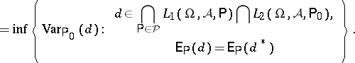 |
Then the covariance method yields again the properties of uniqueness, linearity and closedness (with respect to $\mathsf{P} _ { 0 }$), whereas the property of multiplicativity does not hold, in general, for locally minimum-variance unbiased estimators; this can be illustrated by infinite Bernoulli experiments, where the probability $p$ of success is equal to $1/2$, as follows.
Let ($\Omega , \mathcal{A} , \mathcal{P}$) be the special statistical experiment with $\Omega = \mathbf{N} \cup \{ 0 \}$, $\mathcal{A}$ coinciding with the set of all subsets of $\mathbf{N} \cup \{ 0 \}$, and $\mathcal{P}$ being the set of all binomial distributions $B ( n , 1 / 2 )$ with integer-valued parameter $n \in \mathbf N$ and probability of success $p = 1 / 2$ (cf. also Binomial distribution). Then the covariance method, together with an argument based on interpolation polynomials, yields the following characterization of locally optimal unbiased estimators: $d ^ { * } : \mathbf{N} \cup \{ 0 \} \rightarrow \mathbf{R}$ is locally optimal at $\mathsf{P} _ { n }$ for all $n > \delta$ ($\delta \in \mathbf{N} \cup \{ 0 \}$ fixed) among all estimators $d : \mathbf{N} \cup \{ 0 \} \rightarrow \mathbf{R}$ with $\mathsf{E} _ { \mathsf{P} _ { n } } ( d ) = \mathsf{E} _ { \mathsf{P}_ { n } } ( d ^ { * } )$, $n \in \mathbf N$, if and only if $d ^ { * }$ is a polynomial in $k \in \mathbf{N} \cup \{ 0 \}$ of degree not exceeding $\delta$. In particular, $d ^ { * } : \mathbf{N} \cup \{ 0 \} \rightarrow \mathbf{R}$ is a UMVU estimator if and only if $d ^ { * }$ is already deterministic. Moreover, the property of multiplicativity of locally optimal unbiased estimators is not valid.
There is also the following version of the preceding characterization of locally optimal unbiased estimators for $m$ realizations of independent, identically distributed random variables with some binomial distribution $B ( n , 1 / 2 )$, $n \in \mathbf N$, as follows. Let $\Omega = ( \mathbf{N} \cup \{ 0 \} ) ^ { m }$, let $\mathcal{A}$ be the set of all subsets of $\Omega$, let $\mathcal{P} = \{ \mathsf{P} _ { n } ^ { m } : n \in \mathbf{N} \}$, where  denotes the $m$-fold direct product of $\mathsf{P} _ { n }$ having the binomial distribution $B ( n , 1 / 2 )$. Then $d ^ { * } : \Omega \rightarrow \mathbf{R}$ is locally optimal at
  for all $n > \delta$ ($\delta \in \mathbf{N} \cup \{ 0 \}$ fixed) among all estimators $d : \Omega \rightarrow \mathbf{R}$ with $\mathsf{E} _ { \mathsf{P} _ { n } ^ { m } } ( d ) = \mathsf{E} _ { \mathsf{P} _ { n } ^ { m } } ( d ^ { * } )$, $n \in \mathbf N$, if $d$ is a symmetric polynomial in $( k _ { 1 } , \dots , k _ { m } ) \in ( \mathbf{N} \cup \{ 0 \} ) ^ { m }$ and a polynomial in $k_{j} \in {\bf N} \cup \{ 0 \}$ keeping the remaining variables $k_i$, $i \in \{ 1 , \ldots , m \} \backslash \{ j \}$ fixed, $j = 1 , \ldots , m$, of degree not exceeding $\delta$. In particular, for $m > 1$ the sample mean
\begin{equation*} \frac { 1 } { m } \sum _ { j = 1 } ^ { m } k _ { j } \end{equation*}
is not locally optimal at  for any $n > \delta$ and some fixed $\delta \in \mathbf{N} \cup \{ 0 \}$.
Finally, there are also interesting results about Bernoulli experiments of size $n$ with varying probabilities of success, which, in connection with the randomized response model (cf. [a1]), have the form $p p _ { i } + ( 1 - p ) ( 1 - p _ { i } )$, $i = 1 , \dots , n$, with $p _ { i } \neq 1 / 2$, $i = 1 , \dots , n$, fixed and $p \in [ 0,1 ]$. Then there exists an UMVU estimator for $p$ based on $( x _ { i } , \ldots , x _ { n } ) \in \{ 0,1 \} ^ { n }$ if and only if $p _ { i } = p _ { j }$ or $p _ { i } = 1 - p _ { j }$ for all $i , j \in \{ 1 , \ldots , n \}$. In this case
\begin{equation*} \frac { 1 } { n } \sum _ { j = 1 } ^ { n } \frac { x _ { j } - 1 + p _ { j } } { 2 p _ { j } - 1 } \end{equation*}
is a UMVU estimator for $p$.
If the probabilities of success $p _ { i }$ are functions $f _ { i } : \Theta \rightarrow [ 0,1 ]$, $i = 1 , \dots , n$, with $\Theta$ as parameter space, there exists a symmetric and sufficient data reduction of $( x _ { 1 } , \dots , x _ { n } ) \in \{ 0,1 \} ^ { n }$ if and only if there are functions $g : \Theta \rightarrow \mathbf R$, $h : \{ 1 , \dots , n \} \rightarrow \bf R$ such that
\begin{equation*} f _ { i } ( \vartheta ) = \frac { \operatorname { exp } ( g ( \vartheta ) + h ( i ) ) } { 1 + \operatorname { exp } ( g ( \vartheta ) + h ( i ) ) } , \vartheta \in \Theta , i = 1 , \ldots , n . \end{equation*}
In particular, the sample mean is sufficient in this case.
References
| [a1] | A. Chaudhuri, R. Mukerjee, "Randomized response" , M. Dekker (1988) |
| [a2] | T.S. Ferguson, "Mathematical statistics: a decision theoretic approach" , Acad. Press (1967) |
| [a3] | E.L. Lehmann, "Theory of point estimation" , Wiley (1983) |
Bernoulli experiment. Encyclopedia of Mathematics. URL: http://encyclopediaofmath.org/index.php?title=Bernoulli_experiment&oldid=11211