Bayesian approach, empirical
A statistical interpretation of the Bayesian approach yielding conclusions on unobservable parameters even if their a priori distribution is unknown. Let  be a random vector for which the density
  of the conditional distribution of
  for any given value of the random parameter
  is known. If, as a result of some experiment, only the realization of
  is observed, while the corresponding realization of
  is unknown, and if it is necessary to estimate the value of a given function
  of the non-observed realization, then, in accordance with the empirical Bayesian approach, the conditional mathematical expectation
  should be used as an approximate value
  for
for  . In view of the Bayes formula, this expectation is given by the formula
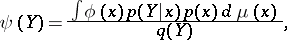 | (1) |
where
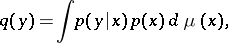 | (2) |
 is the density of the unconditional (a priori) distribution of
  ,
,  is the corresponding
  -finite measure; and the function
  represents the density of the unconditional distribution of
  .
.
If the a priori density  is unknown, it is not possible to compute the values of
  and
and  . However, if a sufficiently large number of realizations of the random variables
  , which are drawn from the distribution with density
  , is known, it is possible to construct a consistent estimator
  , which depends only on
  . S.N. Bernshtein [1] proposed to estimate the value of
  by substituting
  for
for  in (2), finding the solution
  of this integral equation, and then substituting
  and
and  in the right-hand side of (1). However, this method is difficult, since solving this integral equation (2) is an ill-posed problem in numerical mathematics.
In certain special cases the statistical approach may be employed not only to estimate  , but also
  [3]. This is possible if the identity
 | (3) |
involving  and
and  , is true. In (3),
  and
and  are functions which depend on
  only, while
  , being a function of
  , is a probability density (i.e. may be regarded as the density of an arbitrary distribution of some random variable
  for a given value
  ). If (3) is true, the numerator of (1) is equal to the product
 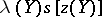 , where
 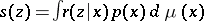 is the density of the unconditional distribution of
  . Thus, if a sufficiently large number of realizations of independent random variables
  with density distribution
  is available, then it is possible to construct a consistent estimator
  for
for  , and hence also to find a consistent estimator
  for
for  :
:
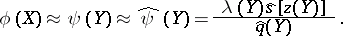 | (4) |
For instance, if one has to estimate  , where
  is a positive integer, and
 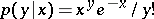 (
( ;
;  ), then
  , where
 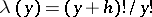 . Since, here,
  , one has
  . Accordingly,
  , i.e. only the sequence of realizations
  is required to find
  . If, on the other hand,
  (
( ;
;  is a positive integer;
  ,
,  ), then
  , where
 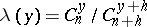 and
and  . For this reason two sequences of empirical values
  and
and  are required in this case to construct
  .
.
This form of the empirical Bayesian approach is applicable to the very narrow class of densities  and functions
  which satisfy condition (3); even if this condition is in fact met, the construction of the estimator (4) is subject to the observability of the random variables
  , the distribution of which usually differs from that of the variables
  which are observed directly. For practical purposes, it is preferable to use the empirical Bayesian approach in a modified form, in which these disadvantages are absent. In this modification the approximation which is constructed does not yield a consistent estimator of
  (such an estimator may even be non-existent), but rather upper and lower estimators of this function, which are found by solving a problem of linear programming, as follows. Let
  and
and  be the constrained minimum and maximum of the linear functional (with respect to the unknown a priori density
  ) in the numerator of (1), calculated under the linear constraints
  ,
, 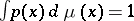 and
and  , where
  is the estimator of
  mentioned above, constructed from the results of the observations
  . One may conclude in such a case that
  , where the probability of the truth of this conclusion tends to one (by virtue of the law of large numbers) as the number of random variables
  , used to construct the estimator
  , increases without limit. Other modifications of the empirical Bayesian approach are also possible — for example, by adding to the last-named condition
  a finite number of conditions of the form
  , where
  are preliminarily given numbers; if
  is replaced by the corresponding confidence bounds for
  , the conditions are obtained in the form of inequalities
  , etc.
In certain cases, which are important in practice, satisfactory majorants, which can be computed without the use of the laborious method of linear programming, can be found for the functions  and
and  (see the example in the entry Sample method which deals with statistical control).
See the entry Discriminant analysis for the applications of the empirical Bayesian approach to hypotheses testing concerning the values of random parameters.
References
| [1] | S.N. Bernshtein, "On "fiducial" probabilities of Fisher" Izv. Akad. Nauk SSSR Ser. Mat. , 5 (1941) pp. 85–94 (In Russian) (English abstract) |
| [2] | L.N. Bol'shev, "Applications of the empirical Bayes approach" , Proc. Internat. Congress Mathematicians (Nice, 1970) , 3 , Gauthier-Villars (1971) pp. 241–247 |
| [3] | H. Robbins, "An empirical Bayes approach to statistics" , Proc. Berkeley Symp. Math. Statist. Probab. , 1 , Berkeley-Los Angeles (1956) pp. 157–163 |
Bayesian approach, empirical. Encyclopedia of Mathematics. URL: http://encyclopediaofmath.org/index.php?title=Bayesian_approach,_empirical&oldid=12163