A priori and a posteriori bounds in matrix computations

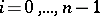
Three sources of errors are behind the lack of accuracy in numerical computations: data errors associated with the physical model, truncation errors when series are truncated to a number of terms, and rounding errors resulting from finite machine precision. Therefore, for the equation in which is a parameter, if an error occurs in , the algorithm returns and not . How much the computed solution differs from is an indication of the computational accuracy of the result. Since is unknown, the norm , taken as an indication of the accuracy, cannot be calculated, and numerical analysts have devised bounds for the latter in terms of the variation in . These bounds are of two types: a priori bounds and a posteriori bounds. The first are applied prior to computation and are usually poor in nature, whereas the second use information extracted from a computation, and are more indicative. In this article, attention is focussed on the most widely available bounds which can be implemented to estimate the accuracy of results and to check the stability of numerical algorithms (cf. also Stability of a computational process).

Linear matrix equations , , .

Assuming that the computed solution is equal to , where and is the error in the solution resulting from a perturbation in and in , the perturbed problem

(a1)

implies, by cancelling equal terms,

(a2)

It follows that for a consistent matrix-vector norm [a1]

(a3)

which implies that under the conditions ,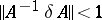

(a4)

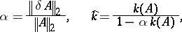
Setting 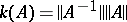, from one finds

(a5)

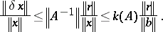
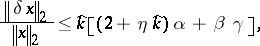
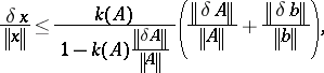
which measures the relative error in the solution resulting from the errors and in the data. Thus, the factor , called the condition number of is the main factor affecting computational accuracy, since by setting , , where is the relative error in the data, it follows that

(a6)

i.e., representing the sensitivity of the solution to relative changes in either or , that is, . So, if and , where is the machine mantissa, the number of significant digits in becomes .

The above analysis lacks accuracy, for the error in is not equal to , since other factors intervene, one of which is the growth factor in the elements associated with the interchange strategy as well as the size of , yet it provides an a priori estimate for the expected accuracy. Before the late J. Wilkinson it was thought that rounding errors can ruin the solution completely; he showed than an upper bound exists for and that fear of obtaining poor results is unwarranted [a2].

On the contrary, one can also reach total machine accuracy. Consider, for example, the matrix

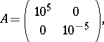, , and , so one expects to loose all significant digits on a -digit machine, contrary to the fact that for any right-hand side , full accuracy in this situation is reached. This led R. Skeel [a3] to consider componentwise estimates of . For , , where stands for the modulus of the vector taken componentwise, one obtains from (a2):

(a7)

giving for , where is the spectral radius, that

(a8)

For relative perturbations in and , this implies that

(a9)

giving

(a10)

which is a better sensitivity criterion. For the above -matrix one has , as expected.

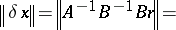
However, a practical bound for the error in relies on information extracted from computation, since it shows the true state of affairs. If is the residual error of the true solution, then by writing one finds , hence the a posteriori bound

(a11)

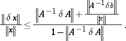
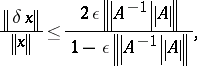
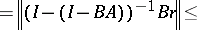
This shows that intervenes also here and that can be found very small, yet is totally inaccurate as a result of the large , [a4]. The above bound can still be improved by noticing that since is unknown and only an approximate inverse matrix of is known, it can be written in the practical form

(a12)

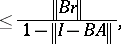provided that .

Although scientists have elaborated on various bounds for estimating the accuracy of their results, the situation is not so bleak, for the above bounds are not the end of the story. After all, can be ameliorated by a technique called the method of iterative refinement, very similar to Newton's method for solving non-linear equations (cf. Newton method). Today it is an available facility in most packages (Linpack, Lapack, etc.) and runs as follows:

a) compute ;

b) solve ;

c) , re-do from a). The algorithm converges very rapidly and .

Finally, accuracy of is not the only issue which matters to users. There is also the question of stability of the algorithms. By the stability of one means that it satisfies the perturbed problem

(a13)

in which and are of the order of the machine allowed uncertainty. An algorithm which returns such that its backward errors and are larger than what is anticipated in terms of the machine eps, is unstable. This is checked using the Oettli–Prager criterion [a5]

(a14)

which has been derived for interval equations but is also suitable for systems subject to uncertainties of the form and . Thus follows the stability criterion ; a result implemented in most available packages by what is called a performance index. (For instance, in the IMSL it is given by

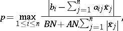(a15)

where , .) If , the solution is stable [a4]. The backward error can be given by , , where is a diagonal matrix and , with .

Linear equations , .

Independent of whether the equations have a unique solution (as in the previous section), more than one solution or no solution (only a least-squares solution), the general solution is given by

(a16)

where is an arbitrary vector and is the Penrose–Moore inverse of , satisfying , , and . For a consistent set of equations the residual , is a special case. The minimal least-squares solution becomes, therefore, . Unlike in the previous section, if undergoes a perturbation , in general cannot be expanded into a Taylor series in ; it does have a Laurent expansion [a4]. For acute perturbations (), from [a6] one finds that

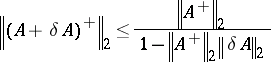(a17)

if

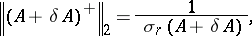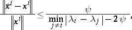
with the singular values of . P. Wedin also showed that for any and ,

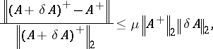(a18)

where has tabulated values for various cases of in relation to and . It therefore follows that the bound for the relative error in is given by

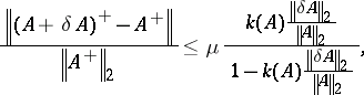(a19)

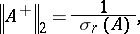
where 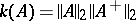is the spectral condition number, which measures the sensitivity of to acute perturbations in . To obtain a bound for one starts with to find that

(a20)

Using a decomposition theorem [a6] for , one finds that [a7]

(a21)

where

(a22)

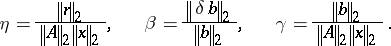Note that the error is dominated by , unlike the bound in (a19), which is dominated by only. For the special case the above expression becomes 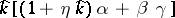. For it becomes . Finally, for it reduces to , which is the situation of the previous section. It should be noted that the above bounds are valid for acute perturbations and that the situation worsens if increases the rank of , in which case the accuracy of deteriorates further as

Again one can follow an iterative scheme of refinement similar to the one mentioned in the previous section to improve on . It runs as follows for the full rank situation:

a) ;

b) ;

c) . The algorithm converges and .

The eigenvalue problem , .

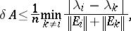
Unlike in the previous sections, a perturbation in affects both the eigenvalue and its corresponding eigenvector . One of the earliest a priori bounds for , where is the eigenvalue of , is the Bauer–Fike theorem [a8]. It states that the eigenvalues of lie in the union of the discs

(a23)

where is the modal matrix of () assuming to be non-defective. The bound follows upon noticing that since

is singular, one has . Writing

one finds that

which implies (a23). The condition number to the problem is therefore of the order of . Indeed, if the above discs are isolated, then and . However, unless is a normal matrix (), the bound in (a23) is known to yield pessimistic results. A more realistic criterion can be obtained. As is singular, then for a vector ,

implying that [a9]

(a24)

which is tighter than (a23) for non-normal matrices. Moreover, (a24) is scale-invariant under the transformation , where is diagonal.

Both the Bauer–Fike bound and the above are valid for the whole spectrum; thus, a group of ill-conditioned eigenvalues affects the bound for the well-conditioned ones. This led Wilkinson to introduce his factors, measuring the sensitivity of the th eigenvalue alone. From first-order perturbation theory one finds, [a1],

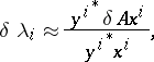(a25)

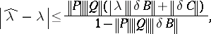
where and are the eigenvector and eigenrow associated with a simple . So, normalizing both of them, becomes the Wilkinson factor and is equal to . However, for a big (a25) does not bound the true shift in . For this one uses a second Bauer–Fike theorem: If

where is the eigenprojection of (i.e., ), then [a8]

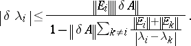(a26)

It follows that represents the sensitivity of to changes in . One can also show that [a10]

(a27)

where bounds the shifts in the eigenvalues. So, the shift in is dependent on the separation of the th eigenvalue from the nearest . Therefore, a matrix has an ill-conditioned eigenvalue problem if or if the discs containing , , intersect as a result of poor separation.

To obtain an a posteriori bound for the error in in terms of the residual one forms , where is an approximate eigenpair. Then , implying

and [a2]

(a28)

For symmetric matrices ; thus, these have well-conditioned eigenproblems. For the non-symmetric case a powerful technique of H. Wielandt [a1] can update by solving iteratively the linear equations

(a29)

and very rapidly.

To check the stability of the solution which satisfies , i.e., , one uses the criterion

(a30)

which asserts that the system is backward stable and there exists a matrix such that is an exact eigenpair of . One can also construct the backwards error in the form , where , satisfying exactly by letting . The above theory is valid for semi-simple eigenvalues only.

The case when is defective (cf. Defective value) is more complicated, since , for a perturbation in , has a Puiseux expansion (cf. Puiseux series) in in powers of , where is the multiplicity of , namely [a1],

(a31)

For an eigenvalue with index (the index is the size of the largest Jordan block) a bound for the shift in is given by [a10]

(a32)

Other bounds.

Modifications of the above cases are often encountered. For instance, the Sylvester equation

(a33)

and its special case , famous in control theory, can be transformed to the case of the first section by considering

(a34)

and a relative perturbation in , , yields with an error [a13]

(a35)

where is the condition number for the problem.

Also, transforming the eigenvalue problem

(a36)

in which , , into a generalized eigenvalue problem , where is the companion matrix for (a36), while using the decomposition 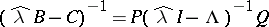, [a1], one obtains [a10]

(a37)

which generalizes (a23).

Many bounds exist for various matrix functions, for instance [a1]

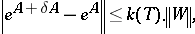(a38)

where

For a general matrix function approximated by another one it can be shown that [a14]

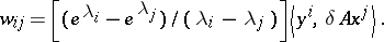
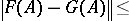(a39)

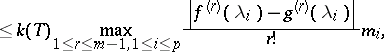where and are scalar functions applied to in the sense that if , then , where is the size of the largest Jordan block associated with , and is the -th derivative of .

References

[a1]	A. Deif, "Advanced matrix theory for scientists and engineers" , Gordon&Breach (1991) (Edition: Second)
[a2]	J. Wilkinson, "The algebraic eigenvalue problem" , Clarendon Press (1965)
[a3]	R. Skeel, "Scaling for numerical stability in Gaussian elimination" J. Assoc. Comput. Mach. , 26 (1979) pp. 494–526
[a4]	A. Deif, "Sensitivity analysis in linear systems" , Springer (1986)
[a5]	W. Oettli, W. Prager, "Compatibility of approximate solution of linear equations with given error bounds for coefficients and right hand sides" Numer. Math. , 6 (1964) pp. 405–409
[a6]	P. Wedin, "Perturbation theory for pseudo-inverses" BIT , 13 (1973) pp. 217–232
[a7]	C. Lawson, R. Hanson, "Solving least-squares problems" , Prentice-Hall (1974)
[a8]	F. Bauer, C. Fike, "Norms and exclusion theorems" Numer. Math. , 2 (1960) pp. 137–141
[a9]	A. Deif, "Realistic a priori and a posteriori bounds for computed eigenvalues" IMA J. Numer. Anal. , 9 (1990) pp. 323–329
[a10]	A. Deif, "Rigorous perturbation bounds for eigenvalues and eigenvectors of a matrix" J. Comput. Appl. Math. , 57 (1995) pp. 403–412
[a11]	G. Stewart, "Introduction to matrix computations" , Acad. Press (1973)
[a12]	G. Stewart, J. Sun, "Matrix perturbation theory" , Acad. Press (1990)
[a13]	A. Deif, N. Seif, S. Hussein, "Sylvester's equation: accuracy and computational stability" J. Comput. Appl. Math. , 61 (1995) pp. 1–11
[a14]	G. Golub, C. van Loan, "Matrix computations" , John Hopkins Univ. Press (1983)