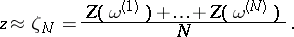
Statistical experiments, method of

A method of numerical calculation that interprets required unknown values as characteristics of a convenient (related) random phenomenon ; this phenomenon is simulated numerically, whereafter the required values are estimated using the simulation of observations of . As a rule, an unknown is sought in the form of the mathematical expectation of some random variable on a probability space that describes , and the independent observations are simulated (see Independence). Then, by the law of large numbers

When 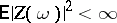, the random error of this formula can be roughly estimated in probability using the Chebyshev inequality or, asymptotically, by the central limit theorem

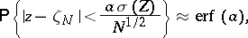(1)

The mathematical expectation can also be estimated "by simulation" , which enables one to make an a posteriori confidence estimation of the accuracy of the calculation. The random phenomenon is usually simulated by means of a sequence of independent random numbers, uniformly distributed on the interval 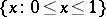(cf. Uniform distribution). For this purpose a measurable mapping from the unit hypercube of countable dimension

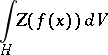
onto is used; , , where the function depends essentially only on coordinates with small indices. The problem thus formally reduces to the calculation of the integral

using the simplest quadrature formula with equal weights and random abscissae . It follows from (1) that the amount of calculation needed to achieve the desired accuracy of the calculation of is determined, given a fixed confidence level , by the product , where is the mathematical expectation of the amount of calculation needed to construct a single realization of ; it increases rapidly as diminishes. A successful choice of a model with sufficiently small is therefore of great value. In particular, it may prove more useful in the original integral representation to make a priori an analytic integration over some of the variables , change some other variables, break the integration cube down into parts, separate the main part of the integral, use groups of dependent points which give the exact quadrature formula for any desired class of functions, etc. The most advantageous "model" can be chosen by estimating roughly the values of and in small preliminary numerical experiments. In making a series of calculations, a noticeable higher degree of accuracy can be obtained by appropriate statistical processing of "observations" and by choosing a corresponding program of "experiments" .

A large class of models used in the method of statistical experiments is related to the scheme of random walks. In the simplest case, is a square matrix of order , , where , , ; , . Consider a Markov random walk through states , with transition probabilities from to , up to the transition at a random -st step to an extra absorbing state , with absorption probability , . Under the assumption that the moving particle changes its weight according to the rule 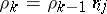, if the -th random transition was from to , , the solution of the equation using a Neumann series can be interpreted coordinatewise as

(2)

where , , . Every "trajectory" is simulated by its sequence of random numbers ; the transition to is completed at the -th step from when . The amount of work involved in constructing the trajectory and calculating the functional from it is proportional to its "length" ; in this scheme .

When simulating random walks in continuous time, the motion must be made discrete. Suppose it is necessary to calculate the fraction of radiation emanating from a sphere of radius , at the centre of which a source is situated. The motion of the radiated particles is rectilinear; on a path with probability a particle interacts with the medium, so that it is absorbed with probability , and is spherically-symmetrically dispersed with probability . The problem is solved by simulating the "particle" trajectories corresponding to the given stochastic differential description of the motion. Instead of breaking down the approximate path of the particle into steps and testing at each step whether interaction has taken place, it is possible, by means of the exponential distribution with density , , to generate the length of an -th random run by means of a single random number, and find the next point of interaction . Moreover, it is possible not to perform a type of interaction with the medium, but to allow for absorption by a weight factor according to the rule . The polar and azimuthal angles of the new direction of the motion are then looked for; is distributed with uniform probability on the interval , and is distributed with uniform probability on the semi-interval . They define the unit vector of the new direction of the motion. The simulation continues until the "particle" leaves the sphere, i.e. until the first event , where is the length of the path up to the boundary of the sphere, . The average weight of the "particles" that have left the sphere provides an estimate of . The integral expression obtained for the required quantity (which also follows from the integral transport equation) can be transformed into an integral along those trajectories that do not leave the sphere. The run must then be performed according to the conditional distribution with density ; the new weight is defined by the rule , and on every trajectory the functional is calculated. Then , where is a continuous function within . In this model, the trajectories are infinite, but the contribution of the later segments (those with a high number, if the segments are numbered beginning with the first one starting at the origin) is small; their simulation can therefore be stopped as soon as by introducing a small systematic error into . The described scheme gives quite good results when . However, for large its use may lead to false conclusions. When , departure from the sphere is rare, and is generally only achieved by trajectories all segments of which are long "on the average" . If is not sufficiently large, then it is highly probable that these a-typical trajectories with a relatively large value of will not occur, and this may lead to underrated (though not to zero) estimates both of the required average and the variance , i.e. an a posteriori measure of the error. Accuracy can be increased here, if an exponential transformation is used, by simulating trajectories by means of the exponential distribution with increased mean run and by compensating this by an extra exponential factor in the weight.

It follows from formula (2) that by solving a system of linear equations via the method of statistical experiments, it is possible to find approximately only one unknown variable without calculating the others. This important property justifies the use of the method of statistical experiments, in spite of its slow convergence, for example, in solving boundary value problems for elliptic differential equations of the second order, when a solution has to be found at only one given point. In particular, for the Laplace equation the solution is written in the form of an integral over Wiener trajectories, i.e. the trajectories of a Brownian motion. The solution of certain boundary value problems for the meta-harmonic (including biharmonic) equations can be written in the form of integrals over the space of random trajectories of a Brownian particle with matrix weight. The simulation of the Brownian trajectories themselves, which undergo an infinitely large number of collisions for any interval of time, can be constructed in large sections by explicit specific methods.

In solving non-linear equations by the method of statistical experiments, more complex models are used of flows of many particles that interact stochastically with the medium and with each other, including cascades of multiplying particles.

Apart from its slow convergence, this method has other shortcomings, including the inadequate reliability of the a posteriori estimation (1) of the random error. It can become less reliable as a result of both "poor quality" (e.g., correlation) of the random numbers used and "non-typicality" (e.g., low probability) of the results of making a main contribution to the integral.

Another name for the method of statistical experiments — the Monte-Carlo method — relates largely to the theory of modifying the method of statistical experiments.

For references, see Monte-Carlo method.

Comments

In the Western literature this method is almost universally known as the Monte-Carlo method.

References

[a1]	B. Ripley, "Stochastic simulation" , Wiley (1987)
[a2]	G. Marsaglia, A. Zaman, W.W. Tsang, "Toward a universal random number generator" Statistics and Prob. Letters , 9 : 1 (1990) pp. 35–39
[a3]	S.M. Ermakov, V.V. Nekrutkin, A.S. Sipin, "Random processes for the classical equations for mathematical physics" , Kluwer (1989) (Translated from Russian)