Fredholm equation, numerical methods
Approximation methods for solving Fredholm integral equations of the second kind, amounting to performing a finite number of operations on numbers.
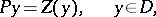
Let
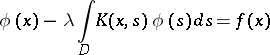 | (1) |
be a Fredholm integral equation of the second kind, where  is a complex number,
  is a known vector function,
  is an unknown vector function,
  is the kernel of equation (1), and
  is a domain in some
  -dimensional Euclidean space. Below it is assumed that
  does not belong to the spectrum of the integral operator with kernel
  (that is, for the given
  equation (1) has a unique solution in some class of functions corresponding to the degree of smoothness of
  ). The expression (1) naturally includes the case of a system of Fredholm equations.
For a general description of the problems of constructing and investigating numerical methods for solving Fredholm equations of the second kind one uses the language of functional analysis. The integral equation (1) can be written as a linear operator equation
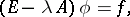 | (2) |
where  is an unknown element of some Banach space
  ,
,  is a given element of
  and
and  is a bounded linear operator from
  to
to  . The operator
  is assumed to act invertibly from
  to
to  . The plan of any numerical method for solving (1) consists of the following. Let
  be a Banach space in some way associated with
  , but, generally speaking, different from it, and let
  be a linear operator from
  to
to  . The equation
 | (3) |
is called an approximating equation for (2). The approximating operator  is usually chosen in such a way that either it may be possible to compute
  directly from (3), or (more commonly) that one may find an approximate solution of (3) of the form
 | (4) |
such that the right-hand side of (4) may be computed in a finite number of arithmetical operations. The expression  denotes performing certain actions on
  and
and  , in particular
  may be a simple operator function of
  (for example,
 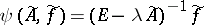 ). The choice of
  ,
,  and
and  , and also of the space
  , is subject to the requirement that
  and the exact solution
  of (1), (2) be (in some sense) close, and is not, generally speaking, unique. Similarly, for a concrete numerical method (a concrete approximation formula for
  ) the choice of
  is not unique. The concrete choice of
  and
and  is dictated by the requirements of "closeness" of
  and
and  , and also by the convenience of the investigation. The specific nature of numerical methods for solving Fredholm equations of the second kind is determined mainly by one or the other concrete approximation of
  by means of
  . So usually an approximation method also gives its name to one or another numerical method for solving (1).
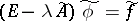
After  ,
,  ,
,  , and
, and  have been chosen, the closeness of
  and
and  (
( ) is established using theorems from the general theory of approximation methods for solving operator equations.
In the case  , in order to establish that
  and
and  are close, it is sufficient to prove that
  is small. For a suitable choice of
  , this can be successfully done for most classical methods for approximately solving Fredholm equations of the second kind.
In the majority of concrete methods the solution of equation (3) can easily be reduced to the solution of a system of linear algebraic equations; in order to construct  in (4), one can make use of some algorithm for solving systems of linear algebraic equations (see Linear algebra, numerical methods in).
The principal methods for constructing approximating operators are:
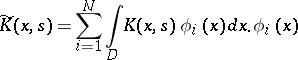
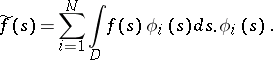
Quadrature methods and generalizations of them. These are the most-widespread methods for approximating the integral operator  in (1). The basis of these methods, which can be applied in the case of continuous
  ,
,  and
and  , consists in replacing the integral (with respect to
  ) in (1) by some quadrature formula with respect to a grid of nodes
  .
.
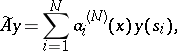
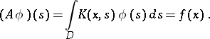
In this case
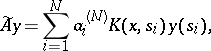 | (5) |
where  are the coefficients of the quadrature formula.
The approximating equation (3) can be regarded as an operator equation in the same space as the basic equation (1) (for example, in the space  of continuous vector functions on
  ). In this case it will have the form
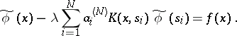 | (6) |
Equation (6) can be reduced to a system of linear algebraic equations in  ,
,  :
:
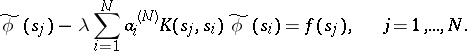 | (7) |
The solution (exact or approximate) of the system (7) gives  .
.
Sometimes one takes the equation (7) itself as approximating (1), and then (7) corresponds to equation (3).
In this approach, the space  is not the same as
  . The space
  may, for example, be identified with the quotient space of
  by the subspace of functions in
  that vanish at the points
  . The method (5) admits various generalizations, which are convenient to use, for example, in the case of a discontinuous
  . In these generalized methods the operator
  has the form
 | (5prm) |
where  are functions associated with the kernel
  .
.
See also Quadrature-sum method.
Methods for replacing the kernel by an approximate one. These make use of an approximating operator  of the form
 |
where  is some function close to
  , but simpler. Most often
  is a degenerate kernel, that is,
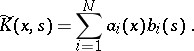 | (8) |
In this case (3) is an integral Fredholm equation with a degenerate kernel (cf. also Degenerate kernels, method of). Its solution reduces to solving a system of linear algebraic equations. However, the matrix entries of the system of equations obtained will be expressed as integrals of known functions, and for a numerical solution of them one must, generally speaking, approximate them by quadrature sums.
There are many ways of making a concrete choice of  by formula (8) (see, for example, Strip method (integral equations)). The theoretical investigation of the closeness of solutions of equations (3) and (1) is usually significantly simpler in these methods than, for example, in quadrature methods, since in most cases one can set
  and the choice of
  is essentially determined directly from the way the problem is posed. If
  and
and  are close, then, as a rule,
  and
and  are close in the norm of
  . However, the practical realization of these methods is in most cases significantly more laborious as compared with quadrature methods and their generalizations.
Projection methods lead to an approximating equation (3) of the form 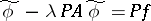 , where
  is a subspace of
  and
and  is the projection onto this subspace. Freedom in the choice of
  ,
,  and even
  itself leads to a large number of concrete projection methods for solving Fredholm integral equations of the second kind. A typical example of a projection method is the Galerkin method. In order to obtain the concrete computational formulas of this method, one must (if possible) treat the integral equation (1) as an operator equation in the Hilbert space
  of functions that are square-integrable in
  , and take as
  the orthogonal projection that associates to a function in
  the
the  -term segment of its Fourier series with respect to some complete orthonormal system of functions
  in
in  .
.
In another interpretation, the Galerkin method is equivalent to that of replacing the kernel by a degenerate one of the form
 |
with a simultaneous replacement of the right-hand side by a function close to it:
 |
As another example of projection methods one can take the collocation method. If  and
and  are continuous functions, then (1) can be regarded as an operator equation (2) in
  — the space of continuous functions on
  . The collocation method corresponds to a choice of
  in the form
 |
where  is the Lagrange interpolation polynomial with respect to some grid of nodes in
  (cf. also Lagrange interpolation formula).
In the practical realization of most projection methods applied to a Fredholm integral equation of the second kind there arise difficulties of the additional approximation of the integrals that appear, which also makes these methods (just like the methods of replacing the kernel by an approximate one) usually more laborious as compared with typical quadrature methods. However, this assertion is relative, since the actual classification of the methods is a matter of convention. For example, the collocation method can be interpreted both as a projection method and as a generalized quadrature method.
Methods for solving the approximating equations. Usually, the solution of an approximating equation (3) reduces to solving a system of linear algebraic equations. One can use methods of successive approximations (the simplest of them) for relatively small  , and with necessary modifications (for example, in the method of averaging functional corrections) one can use them for all
  not belonging to the spectrum of
  .
.
Obtaining a sequence of more accurate approximations. In the theoretical investigation of some numerical method one succeeds in most cases in establishing only the plain fact that the approximations  and
and  converge to a solution of (1) and (2) as
  converges to
  in some sense, and it is extremely rare that one manages to obtain effective estimates of the closeness of
  and
and  to a solution of (1) and (2). To verify the accuracy, one uses in practice a sequence of approximate solutions of (3) with an increasingly-accurate operator
  . In the simplest version of this verification one compares two neighbouring terms in this sequence of approximate solutions and stops obtaining further approximations when the two preceding ones are equal to a given accuracy. The unwieldiness of directly obtaining the terms of such a sequence has been partially surmounted in a variety of algorithms for iteratively obtaining more-accurate approximate solutions. A typical example of such algorithms is the following. If the sequence
  of approximating operators converges in the norm of some Banach function space
  to
to  in (2), then the iterative procedure
 | (9) |
gives a sequence of approximations  that converge to
  , if
, if  converges to
  in norm and if
  is sufficiently close to
  in norm. In using the sequence (9) one requires only one inverse of an operator. The closer
  is to
is to  in norm, the better the convergence is. It is convenient, for example, to choose operators in the form (5). One can in this case establish that
  converges uniformly to
  in
in  , provided that the kernel satisfies certain requirements.
Comments
For some concrete methods, the requirement that  should be small is too strong. Instead, one typically has that (2) is approximated by a sequence
 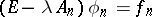 , where
  convergences pointwise to
  and is collectively compact (i.e. for all bounded sets
  ,
,  is compact). Under these assumptions one can prove convergence of the approximate solutions
  and give error bounds. An example where this theory applies is the Nyström method, which consists of solving (7) and then using (6) for extrapolation to all of
  . For the theory of collectively-compact operators and its use in connection with integral equations see [a1].
In collocation methods one can also use interpolation functions other than polynomials, e.g. splines ( "spline collocationspline collocation" ). Because of the better convergence properties of splines (cf. Spline approximation), spline collocation is superior to polynomial collocation.
A variety of concrete numerical methods for Fredholm equations of the second kind are described in [a2] (with Fortran programs), [a3] and [a4]. About numerical methods for solving Fredholm equations if  is an eigen value see [a5], pp. 368ff.
The article above discusses Fredholm integral equations of the second kind only. However, there is also a theory for Fredholm integral equations of the first kind.
Fredholm integral equations of the first kind.
These are equations of the form
 | (a1) |
They are usually ill-posed in the sense that their solution might not exist, not be unique, and will (if it exists) in general depend on  in a discontinuous way (see Ill-posed problems). The notion of solution one commonly uses is the "best-approximate solution"
  , where
  is the Moore–Penrose generalized inverse of
  (see Fredholm equation).
  is in general unbounded. Thus, a "naive" numerical approximation of (a1), e.g. by discretization, will lead to ill-conditioned linear systems. For solving (a1) numerically one uses "regularization methods" (see Regularization method). In general, regularization for (a1) is the replacement of the unbounded operator
  by a parameter-dependent family of bounded linear operators
  (
( ). The "regularized solution" computed with a specific "regularization operator"
  and noisy data
  (
( ) is then
  . The most popular choice for
  is
is  (Tikhonov regularization). Other methods are iterated Tikhonov regularization, iterative methods like Landweber iteration, and truncated singular value expansion, where
 |
Here,  denotes the inner product in
  , and
, and  is a singular system for
  (i.e. the
  are the eigen values of
  ,
,  is a corresponding orthonormal set of eigen vectors,
  ).
).
Convergence rates for regularization methods depend on a priori smoothness assumptions on the data, which also influence the choice of the regularization parameter  . For these questions and details about regularization methods see e.g. [a6], [a7].
For numerical realization, regularization methods have to be combined with projection methods; the latter can also be used directly for regularization (see [a8]).
References
| [a1] | P.M. Anselone, "Collectively compact operator approximation theory and applications to integral equations" , Prentice-Hall (1971) |
| [a2] | K.E. Atkinson, "A survey of numerical methods for the solution of Fredholm integral equations of the second kind" , SIAM (1976) |
| [a3] | C.T.H. Baker, "The numerical treatment of integral equations" , Clarendon Press (1977) pp. Chapt. 4 |
| [a4] | L.M. Delves, J.L. Mohamed, "Computational methods for integral equations" , Cambridge Univ. Press (1985) |
| [a5] | M.Z. Nashed (ed.) , Genealized inverses and applications , Acad. Press (1976) |
| [a6] | H.W. Engl (ed.) C.W. Groetsch (ed.) , Inverse and ill-posed problems , Acad. Press (1987) |
| [a7] | C.W. Groetsch, "The theory of Tikhonov regularization for Fredholm equations of the first kind" , Pitman (1984) |
| [a8] | F. Natterer, "The finite element method for ill-posed problems" RAIRO Anal. Numer. , 11 (1977) pp. 271–278 |
| [a9] | L.V. Kantorovich, V.I. Krylov, "Approximate methods of higher analysis" , Noordhoff (1958) (Translated from Russian) |
| [a10] | I.C. [I.Ts. Gokhberg] Gohberg, I.A. Feld'man, "Convolution equations and projection methods for their solution" , Transl. Math. Monogr. , 41 , Amer. Math. Soc. (1974) (Translated from Russian) |
| [a11] | P.P. Zabreiko (ed.) A.I. Koshelev (ed.) M.A. Krasnoselskii (ed.) S.G. Mikhlin (ed.) L.S. Rakovshchik (ed.) V.Ya. Stet'senko (ed.) T.O. Shaposhnikova (ed.) R.S. Anderssen (ed.) , Integral equations - a reference text , Noordhoff (1975) (Translated from Russian) |
Fredholm equation, numerical methods. Encyclopedia of Mathematics. URL: http://encyclopediaofmath.org/index.php?title=Fredholm_equation,_numerical_methods&oldid=13562