Elimination theory

The theory of eliminating unknowns from systems of algebraic equations. More precisely, suppose one is given a system of equations

(1)

where are polynomials with coefficients in a given field . The problem of eliminating from (1) (the inhomogeneous problem in elimination theory) can be formulated as follows: Find the projection of the set of solutions of (1) on the coordinate space of . If all equations are homogeneous with respect to the set of variables , one also consider the homogeneous problem in elimination theory (the inhomogeneous problem is trivial in this case): Find the projection on the coordinate space of of the set of those solutions of (1) in which not all unknowns are zero.

The inhomogeneous problem can also be regarded as the problem of finding conditions on the coefficients of the system of algebraic equations ensuring that this system is compatible; the homogeneous problem is then that of finding conditions on the coefficients of a system of homogeneous algebraic equations ensuring that this system has a non-zero solution.

The fundamental result of elimination theory is that if is an algebraically closed field, then the solution of the homogeneous problem is an algebraic set, i.e. the set of solutions of a system of algebraic equations, while the solution of the inhomogeneous problem is a constructible set in the sense of algebraic geometry, i.e. a finite union of sets of the form , where and are algebraic sets (cf. also Constructible subset). An explicit solution to problems in elimination theory is known in some of the simplest cases.

1) Consider a system of equations that are linear and homogeneous in , i.e. of the form

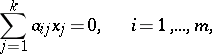(2)

where are polynomials in . For given values of the system (2) has a non-zero solution if and only if the rank of the matrix is less than (cf. Linear equation). The solution of the homogeneous problem now is the set in the coordinate space of described by the vanishing of all minors of rank of .

2) Consider a system of equations that are linear in , i.e. of the form

(3)

where , are polynomials in . Let be the matrix obtained from by addition of the column . For given values of the system (3) is compatible if and only if the rank of equals the rank of . Hence, the result of eliminating from (3) is

where is the set of points at which the rank of is at most , while is the set of points at which the rank of is less than (both and are algebraic sets).

3) Let , let be an algebraically closed field and consider a system of two equations that are homogeneous in , :

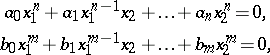(4)

where are polynomials in . For given values of the system (4) has a non-zero solution if and only if the resultant vanishes. Here is given by

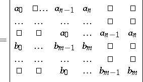( rows of ; rows of ). This also gives a solution of the homogeneous problem in the case considered.

4) Let , let be an algebraically closed field and consider the system of two equations

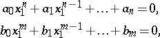(5)

where are polynomials in . For given values of at which either or does not vanish, (5) is a compatible system if and only if

If , one must consider

etc. This makes it possible to describe explicitly the result of eliminating from (5).

The elimination of unknowns from arbitrary systems of algebraic equations can be done successively (i.e. first one eliminates one unknown, then the second, etc.) using the "elementary transformations" described below. Since after eliminating a single unknown one obtains a constructible set instead of an algebraic set, the problem of projecting an arbitrary constructible set in on the coordinate space of must be considered.

Every constructible set can be represented as the union of sets of solutions of a collection of systems of algebraic equations and inequalities. (An algebraic inequality is of the form , where is a polynomial.) An elementary transformation of such a collection is a transformation of one of the following kinds: in one of the systems one adds to one of the equations another equation, multiplied by a polynomial; in a system containing an inequality , one of the equations is multiplied by ; in one of the systems, one adds to one of the inequalities an equation, multiplied by a polynomial; one of the systems is divided into two systems, determined by adding the equation , respectively the inequality , to it ( is an arbitrary polynomial); or, in one of the systems, two inequalities are replaced by their product.

The elementary transformations do not change the union of the sets of solutions of the systems in the original collection. By applying elementary transformations, any collection of algebraic equations and inequalities in unknowns can be reduced to a form in which each of the systems contains at most one equation or inequality containing , and, moreover, together with this equation, , or inequality, , the inequality is contained in it, where , a polynomial in , is the leading coefficient of the expansion of in powers of . If is an algebraically closed field, then by disregarding in the systems the equations and inequalities in thus obtained, one obtains a collection of systems of algebraic and inequalities in . This gives the projection of the set on the coordinate space of .

Sequential elimination of unknowns by elementary transformations allows one to reduce, in principle, the solution of any system of algebraic equations in unknowns to the solution of a number of algebraic equations in one unknown.

References

[1]	W.V.D. Hodge, D. Pedoe, "Methods of algebraic geometry" , 1 , Cambridge Univ. Press (1947)
[2]	B.L. van der Waerden, "Algebra" , 1–2 , Springer (1967–1971) (Translated from German)

Comments

For a non-constructive approach to elimination theory see [a1], § 2C.

References

[a1]	D. Mumford, "Algebraic geometry" , 1. Complex projective varieties , Springer (1976)